theta <- seq(0, 1, by = 0.1)
prior = c(0, 0.024, 0.077, 0.132, 0.173, 0.188, 0.173, 0.132, 0.077, 0.024, 0)
barplot(prior, names.arg = theta, xlab = "theta", ylab = "prior")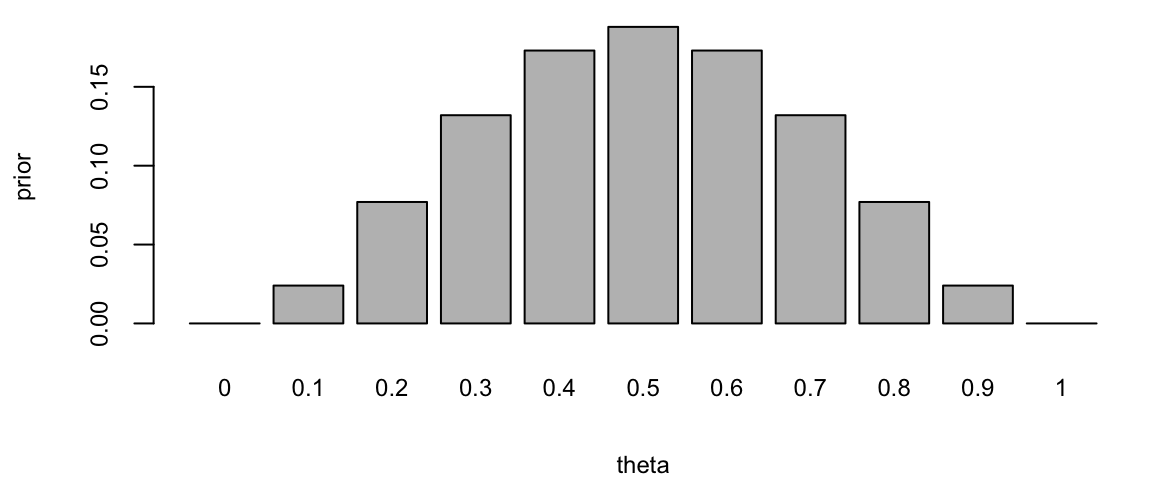
\[ \newcommand{\prob}[1]{\operatorname{P}\left(#1\right)} \newcommand{\Var}[1]{\operatorname{Var}\left(#1\right)} \newcommand{\sd}[1]{\operatorname{sd}\left(#1\right)} \newcommand{\Cor}[1]{\operatorname{Corr}\left(#1\right)} \newcommand{\Cov}[1]{\operatorname{Cov}\left(#1\right)} \newcommand{\E}[1]{\operatorname{E}\left(#1\right)} \newcommand{\defeq}{\overset{\text{\tiny def}}{=}} \DeclareMathOperator*{\argmax}{arg\,max} \DeclareMathOperator*{\argmin}{arg\,min} \DeclareMathOperator*{\mini}{minimize} \]
Bayesian parameter learning is a statistical approach used to update our beliefs about the parameters of a model based on new evidence or data. It is rooted in Bayesian statistics, which is a framework for reasoning about uncertainty and making probabilistic inferences.
In the context of artificial intelligence and statistical modeling, Bayesian parameter learning is particularly relevant when dealing with models that have uncertain or unknown parameters. The goal is to update the probability distribution over the parameters of the model as new data becomes available. The basic steps involved in Bayesian parameter learning include:
Prior Distribution (Prior): Start with a prior distribution that represents your beliefs or knowledge about the parameters before observing any data. This distribution encapsulates the uncertainty about the parameters.
Likelihood Function (Data Likelihood): Specify a likelihood function that describes the probability of observing the given data given the current values of the parameters. This function represents the likelihood of the observed data under different parameter values.
Posterior Distribution (Posterior): Combine the prior distribution and the likelihood function using Bayes’ theorem to obtain the posterior distribution over the parameters. The posterior distribution represents the updated beliefs about the parameters after incorporating the observed data. \[ p( \theta | y ) = \frac{p(y \mid \theta)p( \theta)}{p(y)} \] Here \(\theta\) is the set of model parameters, \(y\) is the observed data. The right hand side \(p( \theta | y )\) is the posterior distribution, \(p(y \mid \theta)\) is the likelihood, \(p(\theta)\) is the prior distribution, and \(p(y)\) is the probability of the observed data (also known as the total probability) given by \[ p(y) = \int p(y \mid \theta)p( \theta)d \theta \]
Posterior as the New Prior (Iterative Process): Use the posterior distribution obtained from one round of observation as the prior distribution for the next round when more data becomes available. This process can be iteratively repeated as new evidence is acquired.
Bayesian Inference: Make predictions or draw inferences by summarizing the information in the posterior distribution. This may involve computing point estimates (e.g., mean, median) or credible intervals that capture a certain percentage of the parameter values.
The key advantage of Bayesian parameter learning is its ability to incorporate prior knowledge and update beliefs based on observed data in a principled manner. It provides a framework for handling uncertainty and expressing the confidence or ambiguity associated with parameter estimates. However, it often requires computational methods, such as Markov Chain Monte Carlo (MCMC) or variational inference, to approximate or sample from the complex posterior distributions.
The Bayes rule allows us to combine the prior distribution and the likelihood function, sometimes we omit the total probability in the denominator on the right hand side and write Bayes rule as \[ \text{Posterior} \propto \text{Likelihood} \times \text{Prior} \]
The choice of prior distribution can significantly impact the ease of computation and the interpretation of the posterior distribution. Conjugate priors are a special type of prior distribution that, when combined with a specific likelihood function, result in a posterior distribution that belongs to the same family as the prior. This property simplifies the computation of the posterior distribution, and allows for analytical solution.
Common examples of conjugate priors include:
Normal distribution with known variance: If the likelihood is a normal distribution with known variance, then a normal distribution is a conjugate prior for the mean.
Binomial distribution: If the likelihood is a binomial distribution, then a beta distribution is a conjugate prior for the probability of success.
Poisson distribution: If the likelihood is a Poisson distribution, then a gamma distribution is a conjugate prior for the rate parameter.
Using conjugate priors simplifies the Bayesian analysis, especially in cases where analytical solutions are desirable. However, the choice of a conjugate prior is often a modeling assumption, and in some cases, non-conjugate priors may be more appropriate for capturing the true underlying uncertainty in the problem.
At the basis of all statistical problems is a potential sample of data, \(y=\left( y_{1},\ldots,y_{T}\right)\), and assumptions over the data generating process such as independence, a model or models, and parameters. How should one view the relationship between models, parameters, and samples of data? How should one define a model and parameters? These questions have fundamental implications for statistical inference and can be answered from different perspectives. This section discusses de Finetti’s representation theorem which provides a formal connection between data, models, and parameters.
To understand the issues, consider the simple example of an experiment consisting of tosses of a simple thumb tack in ideal `laboratory’ conditions. The outcome of the experiment can be defined as a random variable \(y_{i},\) where \(y_{i}=1\) if the \(i^{th}\) toss was a heads (the tack lands on the spike portion) and \(y_{i}=0\) if the tack land tails (on its flat portion). How do we model these random variables? The frequentist or objective approach assumes tosses are independent and identically distributed. In this setting, independence implies that% \[ P\left( y_{2}=1,y_{1}=1\right) =P\left( y_{2}=1\right) P\left( y_{1}=0\right) \text{.}% \]
Given this, are thumbtack tosses independent? Surprisingly, the answer is no. Or at least absolutely not under the current assumptions. Independence implies that \[ P\left( y_{2}=1 \mid y_{1}=1\right) =P\left( y_{2}=1\right) \text{,}% \] which means that observing \(y_{1}=1\) does not effect the probability that \(y_{2}=1\). To see the implications of this simple fact, suppose that the results of 500 tosses were available. If the tosses were independent, then \[ P\left( y_{501}=1\right) =P\left( y_{501}=1\mid {\textstyle\sum\nolimits_{t=1}^{500}}y_{t}=1\right) =P\left( y_{501}=1\mid {\textstyle\sum\nolimits_{t=1}^{500}}y_{t}=499\right) \text{.} \] It is hard to imagine that anyone would believe this–nearly every observer would state that the second probability is near zero and the third probably is near 1 as the first 500 tosses contain a lot of information. Thus, the tosses are not independent.
To see the resolution of this apparent paradox, introduce a parameter, \(\theta\), which is the probability that a thumb tack toss is heads. If \(\theta\) were known, then it is true that, conditional on the value of this parameter, the tosses are independent and \[ P\left( y_{2}=1\mid y_{1}=1,\theta\right) =P\left(y_{2}=1\mid \theta\right) =\theta\text{.} \] Thus, the traditional usage of independence, and independent sampling, requires that `true’ parameter values are known. With unknown probabilities, statements about future tosses are heavily influenced by previous observations, clearly violating the independence assumption. Ironically, if the data was really independent, we would not need samples in the first place to estimate parameters because the probabilities would already be known! Given this, if you were now presented with a thumb tack from a box that was to be repeatedly tossed, do you think that the tosses are independent?
This example highlights the tenuous foundations, an odd circularity, and the internal inconsistency of the frequentist approach that proceeds under the assumption of a fixed `true’ parameter. All frequentist procedures are founded on the assumption of known parameter values: sampling distributions of estimators are computed conditional on \(\theta\); confidence intervals consist of calculations of the form: \(P\left( f\left( y_{1}, \ldots ,y_{T}\right) \in\left( a,b\right) |\theta\right)\); and asymptotics also all rely on the assumption of known parameter values. None of these calculations are possible without assuming the known parameters.
In the frequentist approach, even though the parameter is completely unknown to the researcher, \(\theta\) is not a random variable, does not have a distribution, and therefore inference is not governed by the rules of probability. Given this “fixed, but unknown” definition, it is impossible to discuss concepts like “parameter uncertainty.” This strongly violates our intuition, since things that are not known are typically thought of as random.
The Bayesian approach avoids this internal inconsistency by shedding the strong assumption of independence and replacing it with a weaker and more natural assumption called exchangeability: collection of random variables, \(y_{1}, \ldots ,y_{T}\), is exchangeable if the distribution of \(y_{1}, \ldots ,y_{T}\) is the same as the distribution of any permutation \(y_{\pi_{1}}, \ldots ,y_{\pi_{T}}\), where \(\pi=\left( \pi_{1}, \ldots ,\pi_{T}\right)\) is a permutation of the integers \(1\) to \(T\). In particular, this implies that the order in which the data may arrive does not matter, as their joint density is the same for all potential orderings, and that each observation has the same marginal distribution, \(P\left( y_{i}=1\right) =P\left(y_{j}=1\right)\) for any \(i\) and \(j\). Exchangeability is a weak assumption about symmetry and is weaker than independence, as independent events are always exchangeable, but the converse is not true. Notice the differences between the assumptions in the Bayesian and frequentist approach: the Bayesian makes assumptions over potentially realized data, and there is no need to invent the construct of a fixed but unknown parameter, since exchangeability makes no reference to parameters.
In the case of the tack throwing experiment, exchangeability states that the ordering of heads and tails does not matter. Thus, if the experiment of 8 tosses generated 4 heads, it does not matter if the ordering was \(\left(1,0,1,0,1,0,1,0\right)\) or \(\left( 0,1,1,0,1,0,0,1\right)\). This is a natural assumption about the symmetry of the tack tosses, capturing the idea that the information in any toss or sequence of tosses is the same as any other–the idea of a truly random sample. It is important to note that exchangeability is property that applies prior to viewing the data. After observation, data is no longer a random variable, but a realization of a random variable.
Bruno de Finetti introduced the notion of exchangeability, and then asked a simple question: “What do exchangeable sequences of random variables look like?” The answer to this question is given in the famous de Finetti’s theorem, which also defines models, parameters, and provides important linkages between frequentist and classical statistics.
de Finetti’s representation theorem provides the theoretical connection between data, models, and parameters. It is stated first in the simplest setting, where the observed data takes two values, either zero or one, and then extended below.
Theorem 4.1 (de Finetti’s Representation theorem) Let \(\left( y_{1},y_{2},\ldots\right)\) be an infinite sequence of \(0-1\) exchangeable random variables with joint density \(p\left(y_{1}, \ldots ,y_{T}\right)\). Then there exists a distribution function \(P\) such that
\[
p(y_{1},\ldots,y_{T})=\int\prod_{t=1}^{T}\theta^{y_{t}}(1-\theta)^{1-y_{t}%
}dP(\theta)=\int\prod_{t=1}^{T}p\left( y_{t} \mid \theta\right) dP(\theta)
\tag{4.1}\] where \[
P(\theta)=\underset{T\rightarrow\infty}{\lim}\text{Prob}\left[ \frac{1}%
{T}\sum_{t=1}^{T}y_{t}\leq\theta\right] \text{ and }\theta=\underset {T\rightarrow\infty}{\lim}\frac{1}{T}\sum_{t=1}^{T}y_{t}\text{.}%
\] If the distribution function or measure admits a density with respect to Lebesgue measure, then \(dP(\theta)=p\left( \theta\right) d\theta\).
de Finetti’s representation theorem has profound implications for understanding models from a subjectivist perspective and in relating subjectivist to frequentist theories of inference. The theorem is interpreted as follows:
Under exchangeability, parameters exist, and one can act as if the \(y_{t}\)’\(s\) are drawn independently from a Bernoulli distribution with parameter \(\theta\). That is, they are draws from the model \(p\left(y_{t} \mid \theta\right) =\theta^{y_{t}}(1-\theta)^{1-y_{t}},\) generating a likelihood function \(p\left( y \mid \theta\right) =\prod_{t=1}^{T}p\left(y_{t} \mid \theta\right)\). Formally, the likelihood function is defined via the density \(p\left( y \mid \theta\right)\), viewed as a function of \(\theta\) for a fixed sample \(y=\left( y_{1}, \ldots ,y_{T}\right)\). More “likely” parameter values generate higher likelihood values, thus the name. The maximum likelihood estimate or MLE is \[ \widehat{\theta}=\arg\underset{\theta\in\Theta}{\max}\text{ }p\left(y \mid \theta\right) =\arg\underset{\theta\in\Theta}{\max}\ln p\left(y \mid \theta\right) \text{,}% \] where \(\Theta\) is the parameter space.
Parameters are random variables. The limit \(\theta=\underset {T\rightarrow\infty}{\lim}T^{-1}\sum_{t=1}^{T}y_{t}\) exists but is a random variable. This can be contrasted with the strong law of large numbers that requires independence and implies that \(T^{-1}\sum_{t=1}^{T}y_{t}\) converges almost surely to a fixed value, \(\theta_{0}\). From this, one can interpret a parameter as a limit of observables and justifies the frequentist interpretation of \(\theta\) as a limiting frequency of 1’s.
The distribution \(P\left( \theta\right)\) or density \(p\left(\theta\right)\) can be interpreted as beliefs about the limiting frequency \(\theta\) prior to viewing the data. After viewing the data, beliefs are updated via Bayes rule resulting in the posterior distribution, \[ p\left( \theta \mid y\right) \propto p\left( y \mid \theta\right) p(\theta). \] Since the likelihood function is fixed in this case, any distribution of observed data can be generated by varying the prior distribution.
The main implication of de Finetti’s theorem is a complete justification for Bayesian practice of treating the parameters as random variables and specifying a likelihood and parameter distribution. Stated differently, a `model’ consists of both a likelihood and a prior distribution over the parameters. Thus, parameters as random variables and priors are a necessity for statistical inference, and not some extraneous component motivated by philosophical concerns.
More general versions of de Finetti’s theorem are available. A general version is as follows. If \(\left\{ y_{t}\right\} _{t\geq1}\), \(y_{t}\in\mathbb{R}\), is a sequence of infinitely exchangeable random variables, then there exists a probability measure \(P\) on the space of all distribution functions, such that \[ P(y_{1},\ldots,y_{T})=\int\prod_{t=1}^{T}F\left( y_{t}\right) P(dF) \] with mixing measure \[ P\left( F\right) =\underset{T\rightarrow\infty}{\lim}P(F_{T}), \] where \(F_{T}\) is the empirical distribution of the data. At this level of generality, the distribution function is infinite-dimensional. In practice, additional subjective assumptions are needed that usually restrict the distribution function to finite dimensional spaces, which implies that distribution function is indexed by a parameter vector \(\theta\):% \[ p(y_{1},\ldots,y_{T})=\int\prod_{t=1}^{T}p\left( y_{t} \mid \theta\right) dP\left( \theta\right) \text{.}% \] To operationalize this result, the researcher needs to choose the likelihood function and the prior distribution of the parameters.
At first glance, de Finetti’s theorem may seem to suggest that there is a single model or likelihood function. This is not the case however, as models can be viewed in the same manner as parameters. Denoting a model specification by \(\mathcal{M}\), then de Finetti’s theorem would imply that \[\begin{align*} p(y_{1},\ldots,y_{T}) & =\int\prod_{t=1}^{T}p\left( y_{t} \mid \theta ,\mathcal{M}\right) p\left( \theta \mid \mathcal{M}\right) p\left(\mathcal{M}\right) d\theta d\mathcal{M}\\ & =\int p(y_{1},\ldots,y_{T} \mid \mathcal{M})p\left( \mathcal{M}\right) d\mathcal{M}\text{,}% \end{align*}\] in the case of a continuum of models. Thus, under the mild assumption of exchangeability, it is as if the \(y_{t}\)’\(s\) are generated from \(p\left( y_{t} \mid \theta,\mathcal{M}\right)\), conditional on the random variables \(\theta\) and \(\mathcal{M}\), where \(p\left( \theta \mid \mathcal{M}\right)\) are the beliefs over \(\theta\) in model \(\mathcal{M}\), and \(p\left(\mathcal{M}_{j}\right)\) are the beliefs over model specifications.
The objective approach has been a prevailing one in scientific applications. However, it only applies to events that can be repeated under the same conditions a very large number of times. This is rarely the case in many important applied problems. For example, it is hard to repeat an economic event, such as a Federal Reserve meeting or the economic conditions in 2008 infinitely often. This implies that at best, the frequentist approach is limited to laboratory situations. Even in scientific applications, when we attemt to repeat an experiment multiple times, an objective approach is not guaranteed to work. For example, the failure rate of phase 3 clinical trials in oncology is 60% (Shen et al. (2021),Sun et al. (2022)). Prior to phase 3, the drug is usually tested on several hundred patients.
Subjective probability is a more general definition of probability than the frequentist definition, as it can be used for all types of events, both repeatedable and unrepeatedable events. A subjectivist has no problem discussing the probability a republican president will be re-elected in 2024, even though that event has never occured before and cannot occur again. The main difficulty in operationalizing subjective probability is the process of actually quantifying subjective beliefs into numeric probabilities. This will be discussed below.
Instead of using repetative experiments, subjective probabilities can be measured using betting odds, which have been used for centuries to gauge the uncertainty over an event. The probability attributed to winning a coin toss is revealed by the type of ofdds one would accept to bet. Notice the difference between the frequentist and Bayesian approach. Instead of defining the probabilities via an infinite repeated experiment, the Bayesian approach elicits probabilities from an individual’s observed behavior.
In Bayesian inference, we need to compute the posterior over unknown model parameters \(\theta\), given data \(y\). The posterior density is denoted by \(p(\theta \mid y)\). Here \(y = ( y_1 , \ldots , y_n )\) is high dimensional. Moreover, we need the set of posterior probabilities \(f_B (y) := \pi_{\theta \mid y}(\theta \in B\mid y)\) for all Borel sets \(B\). This problem is computationally hard in high dimensions. Hence, we need dimension reduction for \(y\). The whole idea is to estimate “maps: (a.k.a. transformations/feature extraction) of the output data \(y\) so it is reduced to uniformity.
The dimension reduction problem is to find a low-dimensional representation \(S\) of the data \(y\) that preserves the information in the data.Learning \(S\) can be achieved in a number of ways. Typical architectures include auto-encoders and traditional dimension reduction methods. Polson, Sokolov, and Xu (2021) propose to use a theoretical result of Brillinger methods to perform a linear mapping \(S(y) = W y\) and learn \(W\) using partial least squares (PLS). Nareklishvili, Polson, and Sokolov (2022) extend this to instrumental variables (IV) regression and casual inference problem.
There is a nice connection between the posterior mean and the sufficient statistics, especially minimal sufficient statistics in the exponential family. If there exists a sufficient statistic \(S^*\) for \(\theta\), then Kolmogorov (1942) shows that for almost every \(y\), \(p(\theta\mid y) = p(\theta\mid S^*(y))\) , and further \(S(y) = E_{\pi}(\theta \mid y) = E_{\pi}(\theta \mid S^*(y))\) is a function of \(S^*(y)\). In the special case of an exponential family with minimal sufficient statistic \(S^*\) and parameter \(\theta\), the posterior mean \(S(y) = E_{\pi}(\theta \mid y)\) is a one-to-one function of \(S^*(y)\), and thus is a minimal sufficient statistic.
Deep learners are good interpolators (one of the folklore theorems of machine learning). Hence the set of posteriors \(p(\theta \mid y )\) is characterized by the distributional identity \[ \theta \stackrel{D}{=} H ( S(y_N) , \tau_K ), \; \; \mathrm{where} \; y_N = ( y_1 , \ldots , y_N ) \; \; \tau \sim U(0,1 ) . \]
Summary Statistic: Let \(S(y)\) is sufficient summary statistic in the Bayes sense Kolmogorov (1942), if for every prior \(\pi\) \[ f_B (y) := \pi_{\theta \mid y}(\theta \in B\mid y) = \pi_{\theta \mid s(y)}(\theta \in B\mid s(y)). \] Then we need to use our pattern matching dataset \((y^{(i)} , \theta^{(i)})\) which is simulated from the prior and forward model to “train” the set of functions $ f_B (y)$, where we pick the sets \(B = ( - \infty , q ]\) for a quantile \(q\). Hence, we can then interpolate inbetween.
Estimating the full sequence of functions is then done by interpolating for all Borel sets \(B\) and all new data points \(y\) using a NN architecture and conditional density NN estimation.
The notion of a summary statistic is prevalent in the ABC literature and is tightly related to the notion of a Bayesian sufficient statistic \(S^*\) for \(\theta\), then (Kolmogorov 1942), for almost every \(y\), \[p(\theta \mid Y=y) = p(\theta \mid S^*(Y) = S^*(y) \] Furthermore, \(S(y) = \mathrm{E}\left(\theta \mid Y = y\right) = \mathrm{E}_{p}\left(\theta \mid S^*(Y) = S^*(y)\right)\) is a function of \(S^*(y)\). In the case of exponential family, we have \(S(Y) = \mathrm{E}_{p}\left(\theta | Y \right)\) is a one-to-one function of \(S^*(Y)\), and thus is a minimal sufficient statistic.
Sufficient statistics are generally kept for parametric exponential families, where \(S(\cdot)\) is given by the specification of the probabilistic model. However, many forward models have an implicit likelihood and no such structures. The generalization of sufficiency is a summary statistics (a.k.a. feature extraction/selection in a neural network). Hence, we make the assumption that there exists a set of features such that the dimensionality of the problem is reduced.
The formal model of a coin toss was described by Bernoulli.He modelled the notion of probability for a coin toss, now known as the Bernoulli distribution, there \(X \in \{0,1\}\) and \(P(X=1)=p, P(X=0) = 1-p\). Laplace gave us the principle of insufficient reason: where you would list out the possibilities and then place equal probability on each of the outcomes. Essentially the discrete distribution on the set of possible outcomes.
A Bernoulli trial relates to an experiment with the following conditions
The result of each trial is either a success or failure.
The probability \(p\) of a success is the same for all trials.
The trials are assumed to be independent.
The Bernoulli random variable can take on one of two possible outcomes, typically labeled as “success” and “failure.” It is named after the Swiss mathematician Jacob Bernoulli, who introduced it in the 18th century. The distribution is often denoted by \(\text{Bernoulli}(p)\), where \(p\) is the probability of success.
The probability mass function (PMF) of a Bernoulli distribution is defined as follows: \[ P(X = x) = \begin{cases} p & \text{if } x = 1 \\ 1 - p & \text{if } x = 0 \end{cases} \] The expectation (mean) of a Bernoulli distributed random variable \(X\) is given by: \[\E{X} = p \] Simply speaking, if you are to toss a coin many times, you expect \(p\) heads.
The variance of \(X\) is given by: \[ \Var{X} = p(1-p \]
Example 4.1 (Coin Toss) The quintessential random variable is an outcome of a coin toss. The set of all possible outcomes, known as the sample space, is \(S = \{H,T\}\), and \(p(X = H) = p(X = T) = 1/2\). On the other hand, a single outcome can be an element of many different events. For example, there are four possible outcomes of two coin tosses, HH, TT, HT, TH, which are equally likely with probabilities 1/4. The probability mass function over the number of heads \(X\) out of two coin tosses is
| \(x\) | \(p(x)\) |
|---|---|
| 0 | 1/4 |
| 1 | 1/2 |
| 2 | 1/4 |
Given the probability mass function we can, for example, calculate the probability of at least one head as \(\prob{X \geq 1} = \prob{X =0} + \prob{X =1} = p(0)+p(1) = 3/4\).
The Bernoulli distribution serves as the foundation for more complex distributions, such as the binomial distribution (which models the number of successes in a fixed number of independent Bernoulli trials) and the geometric distribution (which models the number of trials needed to achieve the first success). A Binomial distribution arises from a sequence of Bernoulli trials, and assigns probability to \(X\), which is the number of successes. It’s probability distribution is calculated via: \[ \prob{X=x} = {n \choose x} p^x(1-p)^{n-x}. \] Here \({n \choose x}\) is the combinatorial function, \[ {n \choose x} = \frac{n!}{x!(n-x)!}, \] where \(n!=n(n-1)(n-2)\ldots 2 \cdot 1\) counts the number of ways of getting \(x\) successes in \(n\) trials.
Table below shows the expected value and variance of Binomial random variable.
| Binomial Distribution | Parameters |
|---|---|
| Expected value | \(\mu = \E{X} = n p\) |
| Variance | \(\sigma^2 = \Var{X} = n p ( 1 - p )\) |
For large sample sizes \(n\), this distribution is approximately normal with mean \(np\) and variance of \(np(1-p)\).
Suppose we are about to toss two coins. Let \(X\) denote the number of heads. Then the following table specifies the probability distribution \(p(x)\) for all possible values \(x\) of \(X\). This leads to the following table
| \(x\) | \(\prob{X=x}\) |
|---|---|
| 0 | 1/4 |
| 1 | 1/2 |
| 2 | 1/4 |
Thus, most likely we will see one Head after two tosses. Now, let’s look at a more complex example and introduce our first probability distribution, namely Binomial distribution.
Let \(X\) be the number of heads in three flips. Each possible outcome (“realization”) of \(X\) is an event. Now consider the event of getting only two heads \[ \{ X= 2\} = \{ HHT, HTH, THH \} , \] The probability distribution of \(X\) is Binomial with parameters \(n = 3, p= 1/2\), where \(n\) denotes the sample size (a.k.a. number of trials) and \(p\) is the probability of heads, we have a fair coin. The notation is \(X \sim \mathrm{Bin} \left ( n = 3 , p = \frac{1}{2} \right )\) where the sign \(\sim\) is read as distributed as.
| Result | \(X\) | \(\prob{X=x}\) |
|---|---|---|
| HHH | 3 | \(p^3\) |
| HHT | 2 | \(p^2 ( 1- p)\) |
| HTH | 2 | \(p^2 ( 1 - p)\) |
| THH | 2 | \((1-p)p^2\) |
| HTT | 1 | \(p( 1-p)^2\) |
| THT | 1 | \(p ( 1-p)^2\) |
| TTH | 1 | \((1-p)^2 p\) |
| TTT | 0 | \((1-p)^3\) |
Example 4.2 (Posterior Distribution) What if we gamble against unfair coin flips or the person who performs the flips is trained to get the side he wants? In this case, we need to estimate the probability of heads \(\theta\) from the data. Suppose we have observed 10 flips \[ y = \{H, T, H, H, H, T, H, T, H, H\}, \] and only three of them were tails. What is the probability that the next flip will be tail? The frequency-based answer would be \(3/10 = 0.3\). However, Bayes approach gives us more flexibility. Suppose we have a prior belief that the coin is fair, but we are not sure. We can model this belief by a prior distribution. Let discretize the variable \(\theta\) and assign prior probabilities to each value of \(\theta\) as follows
theta <- seq(0, 1, by = 0.1)
prior = c(0, 0.024, 0.077, 0.132, 0.173, 0.188, 0.173, 0.132, 0.077, 0.024, 0)
barplot(prior, names.arg = theta, xlab = "theta", ylab = "prior")
We put most of the mass to the fair assumption (\(\theta = 0.5\)) and zero mass to the extreme values \(\theta = 0\) and \(\theta = 1\). Our mass is exponentially decaying as we move away from 0.5. This is a reasonable assumption, since we are not sure about the fairness of the coin. Now, we can use Bayes rule to update our prior belief. The posterior distribution is given by \[ p(\theta \mid y) = \frac{p(y \mid \theta) p(\theta)}{p(y)}. \] The denominator is the marginal likelihood, which is given by \[ p(y) = \sum_{\theta} p(y \mid \theta) p(\theta). \] The likelihood is given by the Binomial distribution \[ p(y \mid \theta) = \theta^3 (1 - \theta)^7. \] Notice, that the posterior distribution depends only on the number of positive and negative cases. Those numbers are sufficient for the inference about \(\theta\). The posterior distribution is given by
likelihood <- function(theta, n, Y) {
  theta^Y * (1 - theta)^(n - Y)
}
posterior <- likelihood(theta, 10,3) * prior
posterior <- posterior / sum(posterior) # normalize
barplot(posterior, names.arg = theta, xlab = "theta", ylab = "posterior")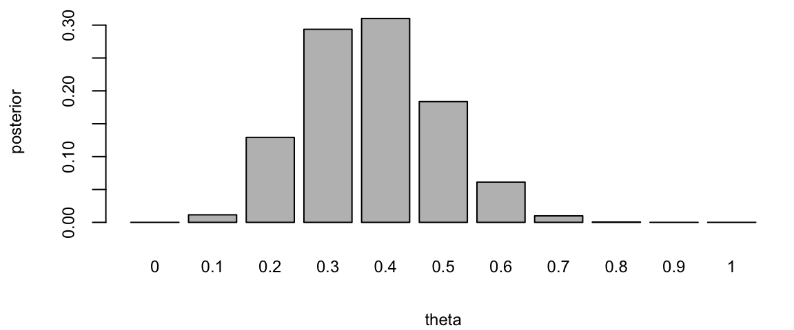
If you are to keep collecting more observations and say observe a sequence of 100 flips, then the posterior distribution will be more concentrated around the value of \(\theta = 0.3\).
posterior <- likelihood(theta, 100,30) * prior
posterior <- posterior / sum(posterior) # normalize
barplot(posterior, names.arg = theta, xlab = "theta", ylab = "posterior")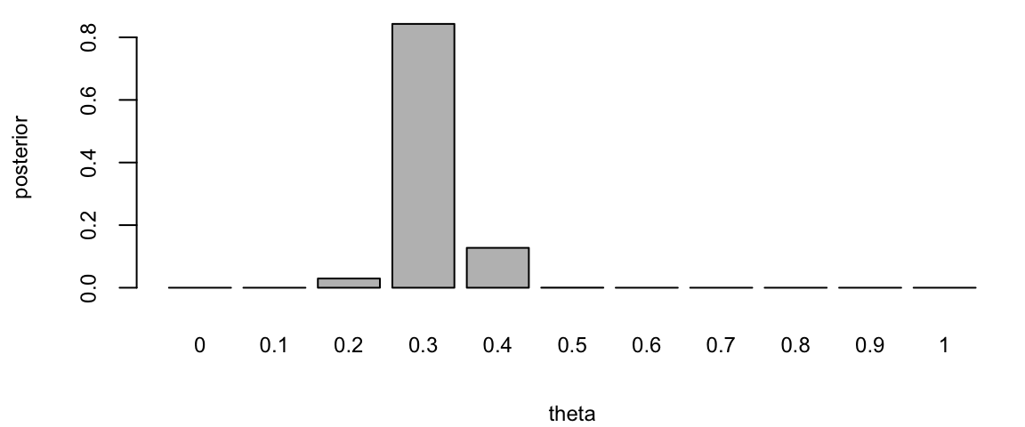
This demonstrates that for large sample sizes, the frequentist approach and Bayes approach agree.
The Beta-Binomial Bayesian model is a statistical model that is used when we are interested in learning about a proportion or probability of success, denoted by \(p\). This model is particularly useful when dealing with binary data such as conversions or clicks in A/B testing.
In the Beta-Binomial model, we assume that the probability of success \(\theta\) in each of \(n\) Bernoulli trials is not fixed but randomly drawn from a Beta distribution. The Beta distribution is defined by two shape parameters, \(\alpha > 0\) and \(\beta > 0\).
The model combines the prior information about \(\theta\) (represented by the Beta distribution) and the observed data (represented by the Binomial distribution) to update our beliefs about \(p\). This is done using Bayes’ Rule, which in this context can be written as: \[ p(\theta \mid Y) = \dfrac{L(\theta \mid Y)p(\theta)}{p(Y)} \] where \(p(\theta)\) is the prior distribution (Beta), \(L(\theta\mid Y)\) is the likelihood function (Binomial), and \(p(\theta\mid Y)\) is the posterior distribution.
The Beta distribution is a family of continuous probability distributions defined on the interval [0,1] in terms of two positive parameters, denoted by alpha (\(\alpha\)) and beta (\(\beta\)), that appear as exponents of the variable and its complement to 1, respectively, and control the shape of the distribution. The Beta distribution is frequently used in Bayesian statistics, empirical Bayes methods, and classical statistics to model random variables with values falling inside a finite interval.
The probability density function (PDF) of the Beta distribution is given by: \[ Beta(x; \alpha, \beta) = \frac{x^{\alpha - 1}(1 - x)^{\beta - 1}}{B(\alpha, \beta)} \]
where \(x \in [0, 1]\), \(\alpha > 0\), \(\beta > 0\), and \(B(\alpha, \beta)\) is the beta function.
The mean and variance of the Beta distribution are given by: \[ \begin{aligned} \mu &= \frac{\alpha}{\alpha + \beta} \\ \sigma^2 &= \frac{\alpha\beta}{(\alpha + \beta)^2(\alpha + \beta + 1)} \end{aligned} \] where \(\mu\) is the mean and \(\sigma^2\) is the variance.
The Beta-Binomial model is one of the simplest Bayesian models and is widely used in various fields including epidemiology, intelligence testing, and marketing. It provides the tools we need to study the proportion of interest, \(p\), in a variety of settings.
The nice property of the Beta-Binomial model is that the posterior \(p(p\mid Y)\) is yet another Beta distribution. Beta is called a conjugate prior for the Binomial likelihood and is a very useful property. Given that we observed \(x\) successful outcome \[ Y = \sum_{i=1}^n Y_i \] the posterior distribution is given by \[ p(\theta\mid Y) =Beta(Y+\alpha, n-Y+\beta) \] where \(p(\theta)\) is the prior distribution (Beta), \(L(\theta\mid Y)\) is the likelihood function (Binomial), and \(p(\theta\mid Y)\) is the posterior distribution. Here the count of successful outcome \(Y\) acts as a sufficient statistic for the parameter \(p\). This means that the posterior distribution depends on the data only through the sufficient statistic \(Y\). This is a very useful property and is a consequence of the conjugacy of the Beta prior and Binomial likelihood.
Example 4.3 (Black Swans) A related problem is the Black Swan inference problem. Suppose that after \(n\) trials where \(n\) is large you have only seen successes and that you assess the probability of the next trial being a success as \((T+1)/(T+2)\) that is, almost certain. This is a model of observing White Swans and having never seen a Black Swan. Taleb (2007) makes it sound as if the rules of probability are not rich enough to be able to handle Black Swan events. There is a related class of problems in finance known as Peso problems where countries decide to devalue their currencies and there is little a prior evidence from recent history that such an event is going to happen.
To obtain such a probability assessment we use a Binomial/Beta conjugate Bayes updating model. The key point is that it can also explain that there is still a large probability of a Black Swan event to happen sometime in the future. Independence model has difficulty doing this.
The Bayes Learning Beta-Binomial model will have no problem. We model with where \(Y_{t}=0\) or \(1\), with probability \(P\left( Y_{t}=1\mid \theta\right) =\theta\). This is the classic Bernoulli “coin-flipping” model and is a component of more general specifications such as regime switching or outlier-type models.
Let \(Y = \sum_{t=1}^{T}y_{t}\) be the number of observed successful outcomes. The likelihood for a sequence of Bernoulli observations is then \[ p\left( y\mid \theta\right) =\prod_{t=1}^{T}p\left( y_{t}\mid \theta\right) =\theta^{Y}\left( 1-\theta\right)^{T-Y}. \] The maximum likelihood estimator is the sample mean, \(\widehat{\theta} = T^{-1}Y\). This makes little sense when you just observe white swans. It predicts \(\hat{\theta} = 1\) and gets shocked when it sees a black swan (zero probability event). Bayes, on the other hand, allows for ‘learning’.
To do this we need prior distribution for the ‘parameter’ \(\theta\). A natural choice is a Beta distribution, denoted by \(\theta\sim\text{Beta}\left( a,A\right)\) with pdf is given by \[ p\left( \theta\mid a,A\right) =\frac{\theta^{a-1}\left( 1-\theta\right)^{A-1}}{B\left( a,A\right) }, \] where \(B\left( \alpha,A\right)\) denotes a Beta function. Since \(p\left( \theta\mid a,A\right)\) is a density and integrates to 1, we have \[ B\left( a,A\right) =\int_{0}^{1}\theta^{a-1}\left( 1-\theta\right) ^{A-1}d\theta . \] Bayes rule then tell us how to combine the likelihood and prior to obtain a posterior distribution, namely \(\theta \mid Y=y\). What do we believe about \(\theta\) given a sequence of. Our predictor rule is then \(P(Y_{t=1} =1 \mid Y=y ) = \mathbb{E}(\theta \mid y)\) it is straightforward to show that the posterior distribution is again a Beta distribution with \[ p\left( \theta\mid y\right) \sim Beta\left( a_{T},A_{T}\right) \; \mathrm{ and} \; a_{T}=a+k , A_{T}=A+T-k. \]
There is a “conjugate” form of the posterior: it is also a Beta distribution and the hyper-parameters \(a_{T}\) and \(A_{T}\) depend on the data only via the sufficient statistics, \(T\) and \(k\). The posterior mean and variance are \[ \mathbb{E}\left[ \theta\mid y\right] =\frac{a_{T}}{a_{T}+A_{T}} \;\text{ and }\; \Var{ \theta\mid y} =\frac{a_{T}A_{T}}{\left( a_{T}+A_{T}\right) ^{2}\left( a_{T}+A_{T}+1\right) }\text{,} \] respectively. This implies that for large samples, \(\E{\theta\mid y} \approx \bar{y} = \widehat{\theta}\), the MLE.
Suppose that after \(n\) trials where \(n\) is large you have only seen successes and that you assess the probability of the next trial being a success as \((T+1)/(T+2)\) that is, almost certain. This is a model of observing White Swans and having never seen a Black Swan. (Taleb, 2008, The Black Swan: the Impact of the Highly Improbable).
To obtain such a probability assessment a natural model is Binomial/Beta conjugate Bayesian updating model. We can access the probability that a black Swan event to happen sometime in the future.
For the purpose of illustration, start with a uniform prior specification, \(\theta \sim \mathcal{U}(0,1)\), then we have the following probability assessment. After \(T\) trials, suppose that we have only seen \(T\) successes, namely, \(( y_1 , \ldots , y_T ) = ( 1 , \ldots , 1 )\). Then you assess the probability of the next trial being a success as \[ p( Y_{T+1} =1 \mid y_1=1 , \ldots , y_T=1 ) = \frac{T+1}{T+2} \] This follows from the mean of the Beta posterior, \[ \theta \mid y \sim \text{Beta}(T+1, T+1), ~ P(Y_{T+1} = 1 \mid y) = \mathbb{E}_{\theta \mid y}\left[P(Y_{T=1} \mid \theta) \right] = \mathbb{E}[\theta \mid y]. \] For large \(T\) this is almost certain.
Now consider a future set of \(n\) trials, where \(n\) is also large. The probability of never seeing a Black Swan is then given by \[ p( y_{T+1} =1 , \ldots , y_{T+n} = 1 \mid y_1=1 , \ldots , y_T=1 ) = \frac{ T+1 }{ T+n+1 } \] For a fixed \(T\), and large \(n\), we have \(\frac{ T+1 }{ T+n+1 } \rightarrow 0\). Hence, we will see a Black Swan event with large probability — we just don’t know when! The exchangeable Beta-Binomial model then implies that a Black Swan event will eventually appear. One shouldn’t be that surprised when it actually happens.
Example 4.4 (Clinical trials) Consdier a problem of designing clinical trials in which \(K\) possible drugs \(a\in 1,\dots,K\) need to be tested. The outcome of the treatment with drug \(a\) is binary \(y(a) \in \{0,1\}\). We use bernoully distribution with mean \(f(a)\) to model the outcome. Thus, the full probabilitic model is described by \(w = f(1),\dots,f(K)\).Say we have observed a sample \(D = \{y_1,\dots,y_n\}\). We would like to compute posterior distribution over \(w\). We start with \(Beta\) prior \[ p(w\mid \alpha,\beta) = \prod_{a=1}^K Beta(w_a\mid \alpha,\beta) \] Then posterior distribution is given by \[ p(w\mid D) = \prod_{a=1}^K Beta(w_a\mid \alpha + n_{a,1},\beta + n_{a,0}) \]
This setrup allows us to perform sequential design of experiment. The simplest version of it is called the Thompson sampling. After observing \(n\) patients, we draw a single sample \(\tilde w\) from the posterior and then maximize the resulting surrogate \[ a_{n+1} = \argmax_{a} f_{\tilde w}(a), ~~~ \tilde{w} \sim p(w\mid D) \]
Example 4.5 (Shrinkage and baseball batting averages) The batter-pitcher match-up is a fundamental element of a baseball game. There are detailed baseball records that are examined regularly by fans and professionals. This data provides a good illustration of Bayesian hierarchical methods. There is a great deal of prior information concerning the overall ability of a player. However, we only see a small amount of data about a particular batter-pitcher match-up. Given the relative small sample size, to determine our optimal estimator we build a hierarchical model taking into account the within pitcher variation.
Let’s analyze the variability in Jeter’s \(2006\) season. Let \(p_{i}\) denote Jeter’s ability against pitcher \(i\) and assume that \(p_{i}\) varies across the population of pitchers according to a particular probability distribution \((p_{i} \mid \alpha,\beta)\sim Be(\alpha,\beta)\). To account for extra-binomial variation we use a hierarchical model for the observed number of hits \(y_{i}\) of the form \[ (y_{i} \mid p_{i})\sim Bin(T_{i},p_{i})\;\;\mathrm{with}\;\;p_{i}\sim Be(\alpha,\beta) \] where \(T_{i}\) is the number of at-bats against pitcher \(i\). A priori we have a prior mean given by \(E(p_{i})=\alpha/(\alpha+\beta)=\bar{p}_{i}\). The extra heterogeneity leads to a prior variance \(Var(p_{i})=\bar{p}_{i}(1-\bar{p}_{i})\phi\) where \(\phi=(\alpha+\beta+1)^{-1}\). Hence \(\phi\) measures how concentrated the beta distribution is around its mean, \(\phi=0\) means highly concentrated and \(\phi=1\) means widely dispersed.
Stern (2007) estimates the parameter \(\hat{\phi} = 0.002\) for Derek Jeter, showing that his ability varies a bit but not very much across the population of pitchers. The effect of the shrinkage is not surprising. The extremes are shrunk the most with the highest degree of shrinkage occurring for the match-ups that have the smallest sample sizes. The amount of shrinkage is related to the large amount of prior information concerning Jeter’s overall batting average. Overall Jeter’s performance is extremely consistent across pitchers as seen from his estimates. Jeter had a season\(.308\) average. We see that his Bayes estimates vary from\(.311\) to\(.327\) and that he is very consistent. If all players had a similar record then the assumption of a constant batting average would make sense.
| Pitcher | At-bats | Hits | ObsAvg | EstAvg | 95% Int | |
|---|---|---|---|---|---|---|
| R. Mendoza | 6 | 5 | .833 | .322 | (.282 | .394) |
| H. Nomo | 20 | 12 | .600 | .326 | (.289 | .407) |
| A.J.Burnett | 5 | 3 | .600 | .320 | (.275 | .381) |
| E. Milton | 28 | 14 | .500 | .324 | (.291 | .397) |
| D. Cone | 8 | 4 | .500 | .320 | (.218 | .381) |
| R. Lopez | 45 | 21 | .467 | .326 | (.291 | .401) |
| K. Escobar | 39 | 16 | .410 | .322 | (.281 | .386) |
| J. Wettland | 5 | 2 | .400 | .318 | (.275 | .375) |
| T. Wakefield | 81 | 26 | .321 | .318 | (.279 | .364) |
| P. Martinez | 83 | 21 | .253 | .312 | (.254 | .347) |
| K. Benson | 8 | 2 | .250 | .317 | (.264 | .368) |
| T. Hudson | 24 | 6 | .250 | .315 | (.260 | .362) |
| J. Smoltz | 5 | 1 | .200 | .314 | (.253 | .355) |
| F. Garcia | 25 | 5 | .200 | .314 | (.253 | .355) |
| B. Radke | 41 | 8 | .195 | .311 | (.247 | .347) |
| D. Kolb | 5 | 0 | .000 | .316 | (.258 | .363) |
| J. Julio | 13 | 0 | .000 | .312 | (.243 | .350 ) |
| Total | 6530 | 2061 | .316 |
Some major league managers believe strongly in the importance of such data (Tony La Russa, Three days in August). One interesting example is the following. On Aug 29, 2006, Kenny Lofton (career\(.299\) average, and current\(.308\) average for \(2006\) season) was facing the pitcher Milton (current record \(1\) for \(19\)). He was rested and replaced by a\(.273\) hitter. Is putting in a weaker player rally a better bet? Was this just an over-reaction to bad luck in the Lofton-Milton match-up? Statistically, from Lofton’s record against Milton we have \(P\left( \leq 1\;\mathrm{hit\;in}\% 19\;\mathrm{attempts} \mid p=0.3\right) =0.01\) an unlikely \(1\)-in-\(100\) event. However, we have not taken into account the multiplicity of different batter-pitcher match-ups. We know that Loftin’s batting percentage will vary across different pitchers, it’s just a question of how much? A hierarchical analysis of Lofton’s variability gave a \(\phi=0.008\) – four times larger than Jeter’s \(\phi=0.002\). Lofton has batting estimates that vary from\(.265\) to\(.340\) with the lowest being against Milton. Hence, the optimal estimate for a pitch against Milton is\(.265<.275\) and resting Lofton against Milton is justified by this analysis.
The Poisson distribution is obtained as a result of the Binomial when \(p\) is small and \(n\) is large. In applications, the Poisson models count data. Suppose we want to model arrival rate of users to one of our stores. Let \(\lambda = np\), which is fixed and take the limit as \(n \rightarrow \infty\). There is a relationship between , \(p(x)\) ans \(p(x+1)\) given by \[ \dfrac{p(x+1)}{p(x)}= \dfrac{\left(\dfrac{n}{x+1}\right)p^{x+1}(1-p)^{n-x-1}}{\left(\dfrac{n}{x}\right)p^{x}(1-p)^{n-x}} \approx \dfrac{np}{x+1} \] If, we approximate \(p(x+1)\approx \lambda p(x)/(x+1)\) with \(\lambda=np\), then we obtain the Poission pdf given by \(p(x) = p(0)\lambda^x/x!\). To ensure that \(\sum_{x=0}^\infty p(x) = 1\), we set \[ f(0) = \dfrac{1}{\sum_{x=0}^{\infty}\lambda^x/x!} = e^{-\lambda}. \] The above equality follows from the power series property of the exponent function \[ e^{\lambda} = \sum_{x=0}^{\infty}\dfrac{\lambda^x}{x!} \] The Poisson distribution counts the occurrence of events. Given a rate parameter, denoted by \(\lambda\), we calculate probabilities as follows \[ p( X = x ) = \frac{ e^{-\lambda} \lambda^x }{x!} \; \mathrm{ where} \; x=0,1,2,3, \ldots \] The mean and variance of the Poisson are given by:
| Poisson Distribution | Parameters |
|---|---|
| Expected value | \(\mu = \E{X} = \lambda\) |
| Variance | \(\sigma^2 = \Var{X} = \lambda\) |
Here \(\lambda\) denotes the rate of occurrence of an event.
Consider the problem of modeling soccer scores in the English Premier League (EPL) games. We use data from Betfair, a website, which posts odds on many football games. The goal is to calculate odds for the possible scores in a match. \[ 0-0, \; 1-0, \; 0-1, \; 1-1, \; 2-0, \ldots \] Another question we might ask, is what’s the odds of a team winning?
This is given by \(P\left ( X> Y \right )\). The odds’s of a draw are given by \(P \left ( X = Y \right )\)?
Professional sports betters rely on sophisticated statistical models to predict the outcomes. Instead, we present a simple, but useful model for predicting outcomes of EPL games. We follow the methodology given in Spiegelhalter and Ng (2009).
First, load the data and then model the number of goals scored using Poisson distribution.
df = read.csv("../../data/epl.csv") #%>% select(home_team_name,away_team_name,home_score,guest_score)
print(help(select))
knitr::kable(head(df))| X | home_team_id | away_team_id | home_team_name | away_team_name | date_string | half_time_score | home_score | guest_score |
|---|---|---|---|---|---|---|---|---|
| 1 | 13 | 26 | Arsenal | Liverpool | 14/08/2016 16:00:00 | 1 : 1 | 3 | 4 |
| 2 | 183 | 32 | Bournemouth | Manchester United | 14/08/2016 13:30:00 | 0 : 1 | 1 | 3 |
| 3 | 184 | 259 | Burnley | Swansea | 13/08/2016 15:00:00 | 0 : 0 | 0 | 1 |
| 4 | 15 | 29 | Chelsea | West Ham | 15/08/2016 20:00:00 | 0 : 0 | 2 | 1 |
| 5 | 162 | 175 | Crystal Palace | West Bromwich Albion | 13/08/2016 15:00:00 | 0 : 0 | 0 | 1 |
| 6 | 31 | 30 | Everton | Tottenham | 13/08/2016 15:00:00 | 1 : 0 | 1 | 1 |
Let’s look at the empirical distribution across the number of goals scored by Manchester United
team_name="Manchester United"
team_for  = c(df[df$home_team_name==team_name,"home_score"],df[df$away_team_name==team_name,"guest_score"])
n = length(team_for)
for_byscore = table(team_for)/n
barplot(for_byscore, col="coral", main="")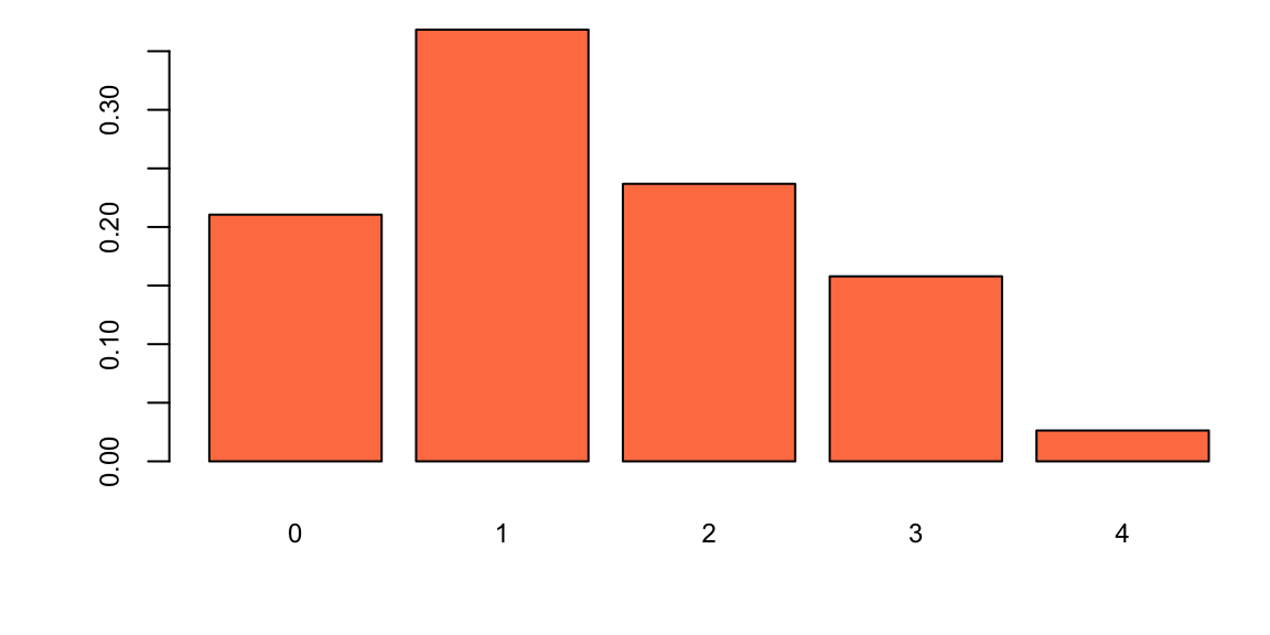
Hence the historical data fits closely to a Poisson distribution, the parameter \(\lambda\) describes the average number of goals scored and we calculate it by calculating the sample mean, the maximum likelihood estimate. A Bayesian method where we assume that \(\lambda\) has a Gamma prior is also available. This lets you incorporate outside information into the predictive model.
lambda_for = mean(team_for)
barplot(rbind(dpois(0:4, lambda = lambda_for),for_byscore),beside = T, col=c("aquamarine3","coral"), xlab="Goals", ylab="probability", main="")
legend("topright", c("Poisson","MU"), pch=15, col=c("aquamarine3", "coral"), bty="n")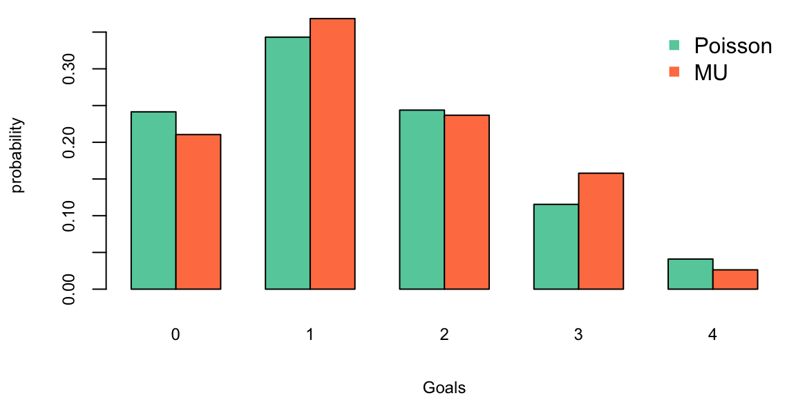
Now we will use Poisson model and Monter Carlo simulations to predict possible outcomes of the MU vs Hull games. First we estimate the rate parameter for goals by MU lmb_mu and goals by Hull lmb_h. Each team played a home and away game with every other team, thus 38 total games was played by all teams. We calculate the average by dividing total number of goals scored by the number of games
sumdf = df %>%
  group_by(home_team_name) %>%
  summarise(Goals_For_Home = sum(home_score)) %>%
  full_join(df %>%
              group_by(away_team_name) %>%
              summarise(Goals_For_Away = sum(guest_score)), by = c("home_team_name" = "away_team_name")
            ) %>%
  full_join(df %>%
              group_by(home_team_name) %>%
              summarise(Goals_Against_Home = sum(guest_score))
            ) %>%
  full_join(df %>%
              group_by(away_team_name) %>%
              summarise(Goals_Against_Away = sum(home_score)), by = c("home_team_name" = "away_team_name")
            ) %>%
  rename(Team=home_team_name)
knitr::kable(sumdf[sumdf$Team %in% c("Manchester United", "Hull"),])| Team | Goals_For_Home | Goals_For_Away | Goals_Against_Home | Goals_Against_Away |
|---|---|---|---|---|
| Hull | 28 | 9 | 35 | 45 |
| Manchester United | 26 | 28 | 12 | 17 |
lmb_mu = (26+28)/38; print(lmb_mu) 1.4lmb_h = (28+9)/38; print(lmb_h) 0.97Now we simulate 100 games between the teams
x = rpois(100,lmb_mu)
y = rpois(100,lmb_h)
sum(x>y) 42sum(x==y) 34knitr::kable(table(x,y))| 0 | 1 | 2 | 3 | 4 | |
|---|---|---|---|---|---|
| 0 | 12 | 6 | 6 | 2 | 0 |
| 1 | 13 | 17 | 5 | 3 | 0 |
| 2 | 7 | 8 | 3 | 1 | 1 |
| 3 | 2 | 3 | 3 | 2 | 0 |
| 4 | 1 | 2 | 1 | 1 | 0 |
| 5 | 0 | 1 | 0 | 0 | 0 |
From our simulaiton that 42 number of times MU wins and 34 there is a draw. The actual outcome was 0-0 (Hull at MU) and 0-1 (Mu at Hull). Thus our model fives a reasonable prediction.
The model can be improved by calculating different averages for home and away games. For example, Hull does much better at home games compared to away games. Further, we can include the characteristics of the opponent team to account for interactions between attack strengh (number of scored) and defence weakness of the opponent. Now we modify our value of expected goals for each of the teams by calculating \[ \hat \lambda = \lambda \times \text{Defense weakness} \]
Let’s model the MU at Hull game. The average away goals for MU \(28/19 = 1.47\) and the defence weakness of Hull is \(36/19 = 1.84\), thus the adjusted expected number of goals to be scored by MU is 2.79. Similarly, the adjusted number of the goals Hull is expected to score is \(28/19 \times 17/19 = 1.32\)
As a result of the simulation, we obtain
set.seed(1)
x <- rpois(100, 28 / 19 * 35 / 19)
y <- rpois(100, 28 / 19 * 17 / 19)
knitr::kable(table(x, y))| 0 | 1 | 2 | 3 | 4 | 5 | |
|---|---|---|---|---|---|---|
| 0 | 1 | 3 | 0 | 0 | 0 | 0 |
| 1 | 3 | 5 | 6 | 1 | 1 | 0 |
| 2 | 4 | 16 | 7 | 3 | 0 | 0 |
| 3 | 6 | 7 | 2 | 3 | 0 | 0 |
| 4 | 4 | 7 | 5 | 2 | 1 | 0 |
| 5 | 2 | 3 | 1 | 2 | 0 | 2 |
| 6 | 1 | 0 | 0 | 1 | 0 | 0 |
| 7 | 1 | 0 | 0 | 0 | 0 | 0 |
image(z = table(x, y), x = 0:7, y = 0:5, xlab = "MU Score", ylab = "Hull Score")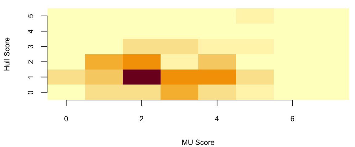
Now we can calculate the number of times MU wins:
sum(x > y) 67A model is only as good as its predictions. Let’s see how our model did in out-of-sample prediction,
Consider a continuous-time stochastic process, \(\left\{ N_{t}\right\} _{t\geq0}\), with \(N_{0}=0\), counting the number of events that have occured up to time \(t\). The process is constant between event times, and jumps by one at event times: \(\Delta N_{t}=N_{t}-N_{t-}=1,\) where \(N_{t-}\) is the limit from the left. The probability of an event over the next short time interval, \(\Delta t\) is \(\lambda\Delta t\), and \(N_{t}\) is called a Poisson process because \[ P\left[ N_{t}=k\right] =\frac{e^{-\lambda t}\left( \lambda t\right) ^{k}}{k!}\text{ for }k=1,\ldots \] which is the Poisson distribution, thus \(N_{t}\sim Poi\left(\lambda t\right)\). A more general version of the Poisson process is a Cox process, or doubly stochastic point process.
Here, there is additional conditioning information in the form of state variables, \(\left\{X_{t}\right\}_{t>0}\). The process now has two sources of randomness, oneassociated with the discontinuous jumps and another in the form of randomstate variables, \(\left\{X_{t}\right\}_{t>0}\), that drive the intensity ofthe process. The intensity of the Cox process is \(\lambda_{t}=\int_{0}^{t}\lambda\left( X_{s}\right) ds\), which is formally defined as \[ P\left[ N_{t}-N_{s}=k \mid \left\{ X_{u}\right\} _{s\leq u\leq t}\right] =\frac{\left( \int_{s}^{t}\lambda\left( X_{s}\right) ds\right) ^{k}\exp\left( -\int_{s}^{t}\lambda\left( X_{s}\right) ds\right)}{k!}, ~ k=0,1,\ldots \] Cox processes are very usefull extensions to Poisson processes and are the basic building blocks of reduced form models of defaultable bonds.
The inference problem is to learn about \(\lambda\) from a continuous-record of observation up to time \(t\). The likelihood function is given by \[ p\left( N_{t}=k \mid \lambda\right) =\frac{\left( \lambda t\right) ^{k}% \exp\left( -\lambda t\right) }{k!}, \] and the MLE is \(\widehat{\lambda}=N_{t}/t\). The MLE has the unattractiveproperty that prior to the first event \(\left\{ t:N_{t}=0\right\}\), the MLEis 0, despite the fact that the model explicitly assumes that events arepossible. This problem often arises in credit risk contexts, where it wouldseem odd to assume that the probability of default is zero just because adefault has not yet occured.
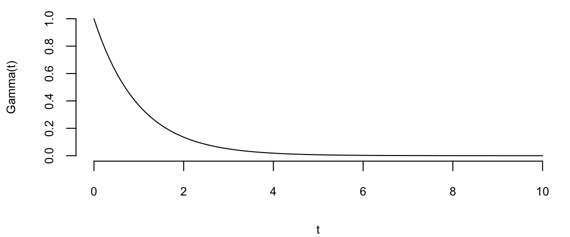
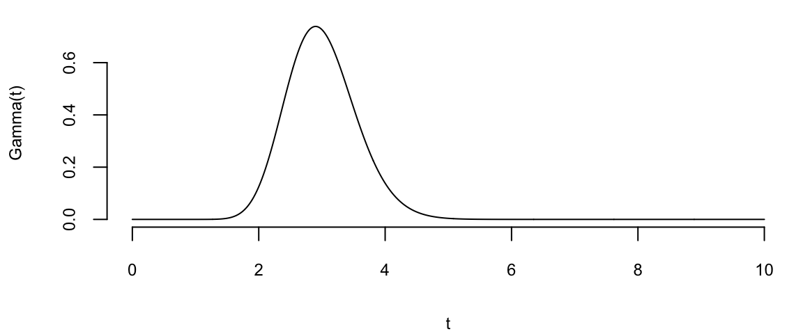
A natural prior for this model is the Gamma distribution, which has the following pdf \[ p\left( \lambda \mid a,A\right) =\frac{A^{a}}{\Gamma(A) }% x^{a-1}\exp\left( -Ax\right) \text{.}% \tag{4.2}\] Like the beta distribution, a Gamma prior distribution allows for a variety of prior shapes and is parameterized by two hyperparameters. Combining the prior and likelihood, the posterior is also Gamma: \[ p\left( \lambda \mid N_{t}\right) \propto\frac{\left( \lambda\right) ^{N_{t}+a-1}\exp\left( -\lambda\left( t+A\right) \right) }{N_{t}!}% \sim\mathcal{G}\left( a_{t},A_{t}\right) , \] where \(a_{t}=N_{t}+a\) and \(A_{t}=t+A\). The expected intensity, based on information up to time \(t\), is \[ \mathbb{E}\left[ \lambda \mid N_{t}\right] =\frac{a_{t}}{A_{t}}=\frac{N_{t}% +a}{t+A}=w_{t}\frac{N_{t}}{t}+\left( 1-w_{t}\right) \frac{a}{A}, \] where the second line expresses the posterior mean in shrinkage form as a weighted average of the MLE and the prior mean where \(w_{t}=t/(t+A)\). In large samples, \(w_{t}\rightarrow1\) and \(E\left( \lambda \mid N_{t}\right) \approx N_{t}/t=\widehat{\lambda}\).
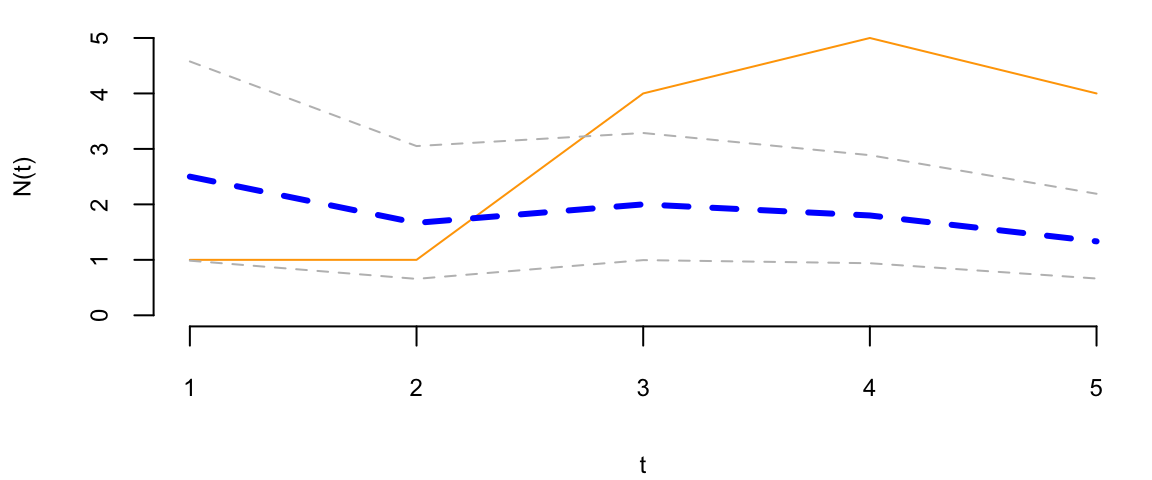
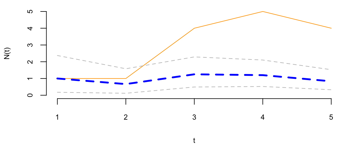
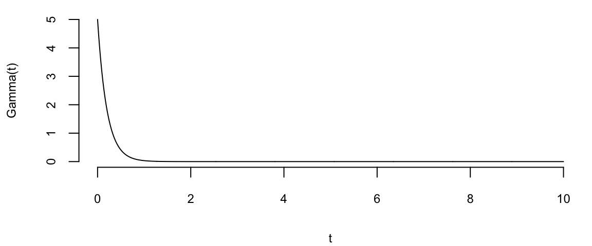
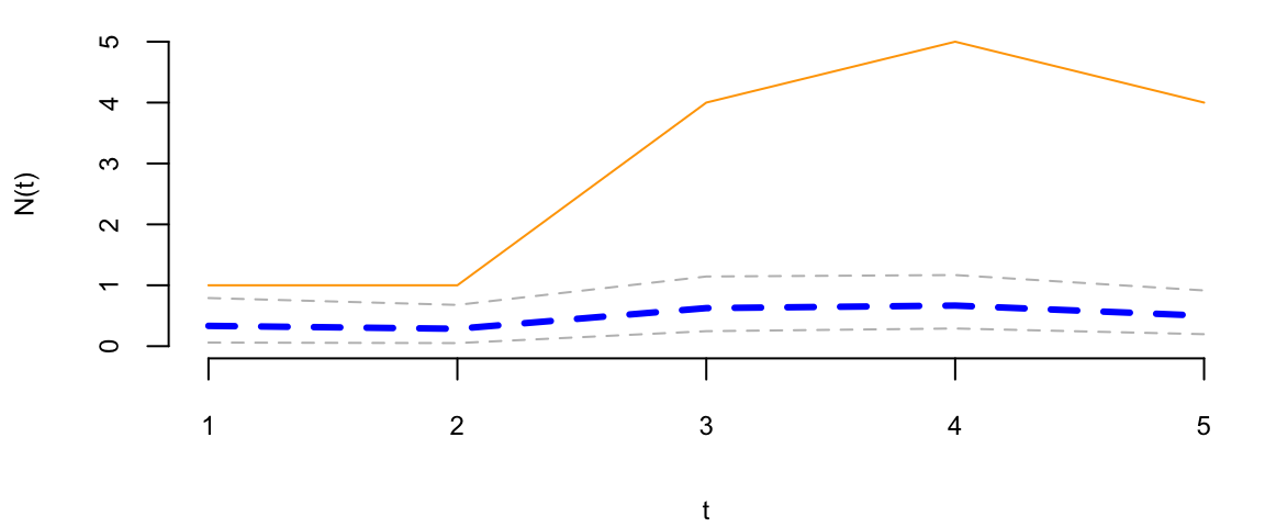
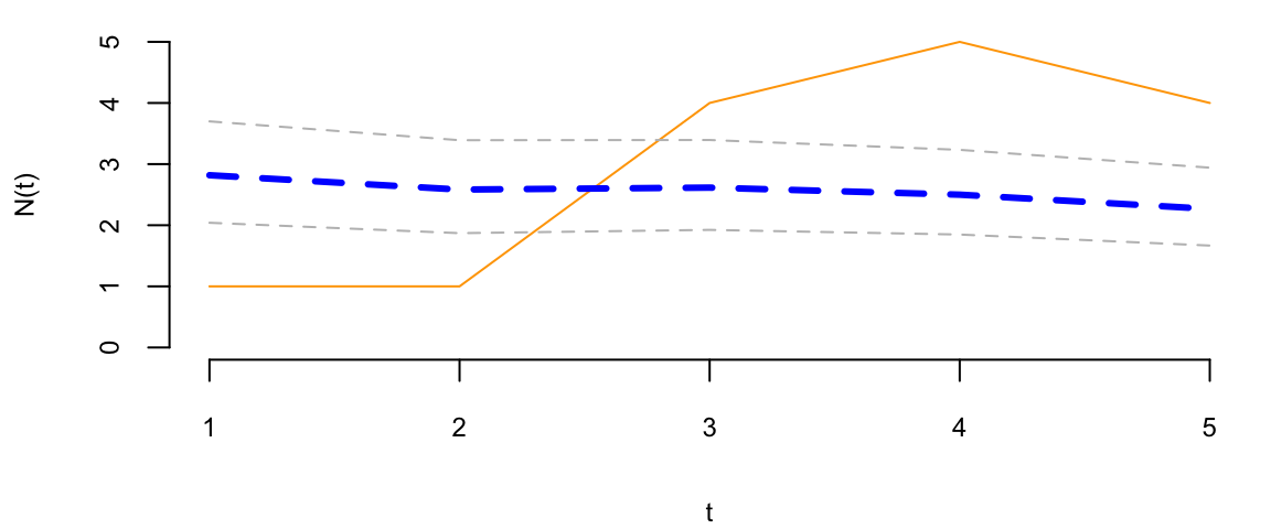
To understand the updating mechanics, Figure 4.1 (right column) displays a simulated sample path, posterior means, and (5%,95%) posterior quantiles for various prior configurations. In this case, time is measured in years and the intensity used to simulate the data is \(\lambda=1\), implying on average one event per year. The four prior configurations embody different beliefs. In the first case, in the middle left panel, \(a=4\) and \(A=1\), captures a high-activity prior, that posits that jumps occur, on average, four times per year, and there is substantial prior uncertainty over the arrival rate as the (5%,95%) prior quantiles are (1.75,6.7). In the second case, in the middle right panel, captures a prior that is centered over the true value with modest prior uncertainty. The third case, the bottom left panel, captures a low-activity prior, with a prior mean of 0.2 jumps/year. The fouth case captures a dogmatic prior, that posits that jumps occur three times per year, with high confidence in these beliefs.
The priors were chosen to highlight different potential paths for Bayesian learning. The first thing to note from the priors is the discontinuity upward at event times, and the exponential decrease during periods of no events, both of which are generic properties of Bayesian learning in this model. If one thinks of the events as rare, this implies rapid revisions in beliefs at event times and a constant drop in estimates of the intensity in periods of no events. For the high-activity prior and the sample path observed, the posterior begins well above \(\lambda=1\), and slowly decreases, getting close to \(\lambda=1\) at the end of the sample. This can be somewhat contrasted with the low-activity prior, which has drastic revisisions upward at jump times. In the dogmatic case, there is little updating at event times. The prior parameters control how rapidly beliefs change, with noticeable differences across the priors.%
set.seed(8) # Ovi
t = 1:5
lmb = 1
N = rpois(5,t*lmb)

# A: rate (beta), a: shape (alpha)
plotgamma = function(a,A,N) {
    x = seq(0,10,0.01)
    plot(x,dgamma(x,a,A),type="l",xlab="t",ylab="Gamma(t)")
    at = N+a
    At = t+A
    mean = at/At
    plot(N, type='l', col="orange", ylim=c(0,5), xlab="t", ylab="N(t)")
    lines(mean, col="blue", lwd=3, lty=2)
    lines(qgamma(0.05,at,At), col="grey", lwd=1, lty=2)
    lines(qgamma(0.95,at,At), col="grey", lwd=1, lty=2)
}
plotgamma(a=4,A=1, N)
plotgamma(a=1,A=1, N)
plotgamma(a=1,A=5, N)
plotgamma(a=30,A=10, N)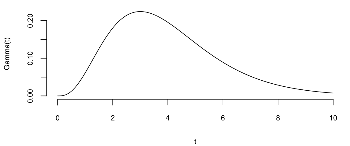
Poisson event models are often embedded as portion of more complicated model to capture rare events such as stock market crashes, volatility surges, currency revaluations, or defaults. In these cases, prior distributions are often important–even essential–since it is common to build models with events that could, but have not yet occurred. These events are often called ‘Peso’ events. For example, in the case of modeling corporate defaults a researcher wants to allow for a jump to default. This requires positing a prior distribution that places non-zero probability on an event occuring. Classical statistical methods have difficulties dealing with these situations since the MLE of the jump probability is zero, until the first event occurs.
The Normal or Gaussian distribution is central to probability and statistical inference. Suppose that we are trying to predict tomorrow’s return on the S&P500. There’s a number of questions that come to mind
What is the random variable of interest?
How can we describe our uncertainty about tomorrow’s outcome?
Instead of listing all possible values we’ll work with intervals instead. The probability of an interval is defined by the area under the probability density function.
Returns are are continuous (as opposed to discrete) random variables. Hence a normal distribution would be appropriate - but on what scale? We will see that on the log-scale a Normal distribution provides a good approximation.
The most widely used model for a continuous random variable is the normal distribution. Standard normal random variable \(Z\) has the following properties
The standard Normal has mean \(0\) and has a variance \(1\), and is written as \[ Z \sim N(0,1) \] Then, we have the probability statements of interest \[\begin{align*} P{-1 <Z< 1} &=0.68\\ P{-1.96 <Z< 1.96} &=0.95\\ \end{align*}\]
In R, we can find probabilities
pnorm(1.96) 0.98and quantiles
qnorm(0.9750) 2The quantile function qnorm is the inverse of pnorm.
A random variable that follows normal distribution with general mean and variance \(X \sim \mbox{N}(\mu, \sigma^2)\), has the following properties \[\begin{align*} p(\mu - 2.58 \sigma < X < \mu + 2.58 \sigma) &=& 0.99 \\ p(\mu - 1.96 \sigma < X < \mu + 1.96 \sigma) &=& 0.95 \, . \end{align*}\] The chance that \(X\) will be within \(2.58 \sigma\) of its mean is \(99\%\), and the chance that it will be within \(2\sigma\) of its mean is about \(95\%\).
The probability model is written \(X \sim N(\mu,\sigma^2)\), where \(\mu\) is the mean, \(\sigma^2\) is the variance. This can be transformed to a standardized normal via \[ Z =\frac{X-\mu}{\sigma} \sim N(0,1). \] For a normal distribution, we know that \(X \in [\mu-1.96\sigma,\mu+1.96\sigma]\) with probability 95%. We can make similar claims for any other distribution using the Chebyshev’s empirical rule, which is valid for any population:
At least 75% probability lies within 2\(\sigma\) of the mean \(\mu\)
At least 89% lies within 3\(\sigma\) of the mean \(\mu\)
At least \(100(1-1/m^2)\)% lies within \(m\times \sigma\) of the mean \(\mu\).
This also holds true for the Normal distribution. The percentages are \(95\)%, \(99\)% and \(99.99\)%.
Example 4.6 (Stock market crash 1987) Prior to the October, 1987 crash SP500 monthly returns were 1.2% with a risk/volatility of 4.3%. The question is how extreme was the 1987 crash of \(-21.76\)%? \[ X \sim N \left(1.2, 4.3^2 \right ) \] This probability distribution can be standardized to yield \[ Z =\frac{X-\mu}{\sigma} = \frac{X - 1.2}{4.3} \sim N(0,1) . \] Now,, we calculate the observed \(Z\), given the outcome of the crash event \[ Z = \frac{-0.2176 - 0.012}{0.043} = -5.27 \] That’s is \(5\)-sigma event in terms of the distribution of \(X\). Meaning that -0.2176 is 5 standard diviations away from the mean. Under a normal model that is equivalent to \(P(X < -0.2176)\) = 4.66^{-8}.
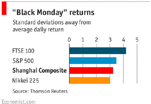
On August 24th, 2015, Chinese equities ended down $- 8.5 $% (Black Monday). In the last \(25\) years, average is $0.09 $% with a volatility of $2.6 $%, and \(56\)% time close within one standard deviation. SP500, average is \(0.03\)% with a volatility of \(1.1\)%. \(74\)% time close within one standard deviation
The method of estimating the parameters of the normal distribution we used above (sample mean and variance) is called the method of moments, meaning that we estimate the variance and the mean (first two moments of a distribution) by simply calculating those from the observed sample.
We can formalise this fully in the Normal/ Normal Bayes learning model as follows. We add prior \(\theta\sim \mathcal{N}(\theta_0, \tau^2)\) and likelihood, \(p(y \mid \theta, \sigma^2) \equiv p(\bar{y} \mid \theta, \sigma^2)\).
Notice that we have reduced the data by sufficiency and we only need \(\bar{y}\) rather than the full dataset \(\left(y_1,y_2, \ldots, y_n \right)\). The Normal/ Normal Bayesian learning model provides the basis for shrinkage estimation of multiply means and the basis of the Kalman filter for dynamically tracking a path of an object.
The Kalman filter is arguable the most common application of Bayesian inference. The Kalman filter assumes a linear and Gaussian state spacemodel: \[ y_{t}=x_{t}+\sigma\varepsilon_{t}^{y}\text{ and }x_{t}=x_{t-1}+\sigma _{x}\varepsilon_{t}^{x}, \] where \(\varepsilon_{t}^{y}\) and \(\varepsilon_{t}^{x}\) are i.i.d. standard normal and \(\sigma\) and \(\sigma_{x}\) are known. The observation equation posits that the observed data, \(y_{t}\), consists of the random-walk latent state, \(x_{t}\), that is polluted by noise, \(\sigma\varepsilon_{t}^{y}\). \(\sigma_{x}/\sigma\), the `signal-to-noise’ ratio, measures the information content of the signal. As \(\sigma\) increases relatively to \(\sigma_{x}\), the observations become noisier and less informative. The model is initialized via a prior distribution over \(x_{0}\), which is for analytical tractability must be normally distributed, \(x_{0}\sim\mathcal{N}\left( \mu_{0},\sigma_{0}^{2}\right)\). Numerical examples of this model will be given later.
The posterior distribution solves the filtering problem and is defined recursively via Bayes rule: \[ p\left( x_{t+1} \mid y^{t+1}\right) =\frac{p\left( y_{t+1} \mid x_{t+1}\right) p\left( x_{t+1} \mid y^{t}\right) }{p\left( y_{t+1} \mid y^{t}\right) }\propto p\left( y_{t+1} \mid x_{t+1}\right) p\left( x_{t+1} \mid y^{t}\right) \text{.}% \] and the likelihood function, \(p\left( y_{t+1} \mid x_{t+1}\right)\). The predictive distribution summarizes all of the information about \(x_{t+1}\) based on lagged observations. The likelihood function summarizes the new information in \(y_{t+1}\) about \(x_{t+1}\).
The Kalman filter relies on an inductive argument: assume that \(p\left( x_{t} \mid y^{t}\right) \sim\mathcal{N}\left( \mu_{t},\sigma_{t}^{2}\right)\) and then verify that \(p\left( x_{t+1} \mid y^{t+1}\right) \sim\mathcal{N}\left( \mu_{t+1},\sigma_{t+1}^{2}\right)\) with analytical expressions for the hyperparameters. To verify, note that since \(p\left(x_{t} \mid y^{t}\right) \sim\mathcal{N}\left( \mu_{t},\sigma_{t}^{2}\right)\), \(x_{t}=\mu_{t}+\sigma_{t}\eta_{t}\) for some standard normal \(\eta_{t}\). Substituting into the state evolution, the predictive is \(x_{t+1} \mid y^{t}\sim\mathcal{N}\left( \mu_{t},\sigma_{t}^{2}+\sigma_{x}^{2}\right)\). Since \(p\left( y_{t+1} \mid x_{t+1}\right) \sim\mathcal{N}\left(x_{t+1},\sigma^{2}\right)\), the posterior is \[\begin{align*} p\left( x_{t+1} \mid y^{t+1}\right) & \propto p\left( y_{t+1} \mid x_{t+1}\right) p\left( x_{t+1} \mid y^{t}\right) \propto\exp\left[ -\frac{1}{2}\left( \frac{\left( y_{t+1}-x_{t+1}\right) ^{2}}{\sigma^{2}}+\frac{\left( x_{t+1}-\mu_{t}\right) ^{2}}{\sigma_{t}^{2}+\sigma_{x}^{2}}\right) \right] \\ & \propto\exp\left( -\frac{1}{2}\frac{\left( x_{t+1}-\mu_{t+1}\right) ^{2}}{\sigma_{t+1}^{2}}\right) \end{align*}\] where \(\mu_{t+1}\) and \(\sigma_{t+1}^{2}\) are computed by completing the square: \[\begin{equation} \frac{\mu_{t+1}}{\sigma_{t+1}^{2}}=\frac{y_{t+1}}{\sigma^{2}}+\frac{\mu_{t}% }{\sigma_{t}^{2}+\sigma_{x}^{2}}\text{ and }\frac{1}{\sigma_{t+1}^{2}}% =\frac{1}{\sigma^{2}}+\frac{1}{\sigma_{t}^{2}+\sigma_{x}^{2}}\text{.}\nonumber \end{equation}\] Here, inference on \(x_{t}\) is merely running the Kalman filter, that is, sequential computing \(\mu_{t}\) and \(\sigma_{t}^{2}\), which are state suffiicent statistics.
The Kalman filter provides an excellent example of the mechanics of Bayesian inference: given a prior and likelihood, compute the posterior distribution. In this setting, it is hard to imagine an more intuitive or alternative approach. The same approach applied to learning fixed static parameters. In this case, \(y_{t}=\mu+\sigma\varepsilon_{t},\) where \(\mu\sim\mathcal{N}\left( \mu_{0},\sigma_{0}^{2}\right)\) is the initial distribution. Using the same arguments as above, it is easy to show that \(p\left(\mu \mid y^{t+1}\right) \sim\mathcal{N}\left( \mu_{t+1},\sigma_{t+1}^{2}\right)\), where \[\begin{align*} \frac{\mu_{t+1}}{\sigma_{t+1}^{2}} & =\left( \frac{y_{t+1}}{\sigma^{2}}+\frac{\mu_{t}}{\sigma_{t}^{2}}\right) =\frac{\left( t+1\right) \overline{y}_{t+1}}{\sigma^{2}}+\frac{\mu_{0}}{\sigma_{0}^{2}}\text{,}\\ \frac{1}{\sigma_{t+1}^{2}} & =\frac{1}{\sigma^{2}}+\frac{1}{\sigma_{t}^{2}}=\frac{\left( t+1\right) }{\sigma^{2}}+\frac{1}{\sigma_{0}^{2}}\text{,} \end{align*}\] and \(\overline{y}_{t}=t^{-1}\sum_{t=1}^{t}y_{t}\).
Now, given this example, the same statements can be posed as in the state variable learning problem: it is hard to think of a more intuitive or alternative approach for sequential learning. In this case, researchers often have different feelings about assuming a prior distribution over the state variable and a parameter. In the state filtering problem, it is difficult to separate the prior distribution and the likelihood. In fact, one could view the intial distribution over \(x_{0}\), the linear evolution for the state variable, and the Gaussian errors as the “prior” distribution.
Let’s look at stylezed example, assuming the proir distribution \(\theta \sim N(-1,1)\), say we observed \(y=2\) and we want to update our beliefs about \(\theta\). The likelihood function is \(p(y \mid \theta) = N(\theta,2)\), and the posterior distribution is \[ p(\theta \mid y) \propto p(y \mid \theta) p(\theta) = N(\theta,2) N(-1,1) = N(\theta, 1/2). \] Graphically we can represent this as follows
# The prior distribution
mu0 = -1
sigma0 = 1
y = seq(-4,10,0.01)
plot(y,dnorm(y,mu0,sigma0),type="l",xlab="x",ylab="p(x)",lwd=2,col="blue",ylim=c(0,0.5))
# The likelihood function
ybar = 2
sigma = 2
lines(y,dnorm(y,ybar,sigma),type="l",lwd=2,col="red")
# The posterior distribution
mu1 = (mu0/sigma0^2 + ybar/sigma^2)/(1/sigma0^2 + 1/sigma^2)
sigma1 = sqrt(1/(1/sigma0^2 + 1/sigma^2))
lines(y,dnorm(y,mu1,sigma1),type="l",lwd=2,col="green")
# legend
legend("topright", c("Prior"," Data (Likelihood)","Posterior"), pch=15, col=c("blue", "red", "green"), bty="n")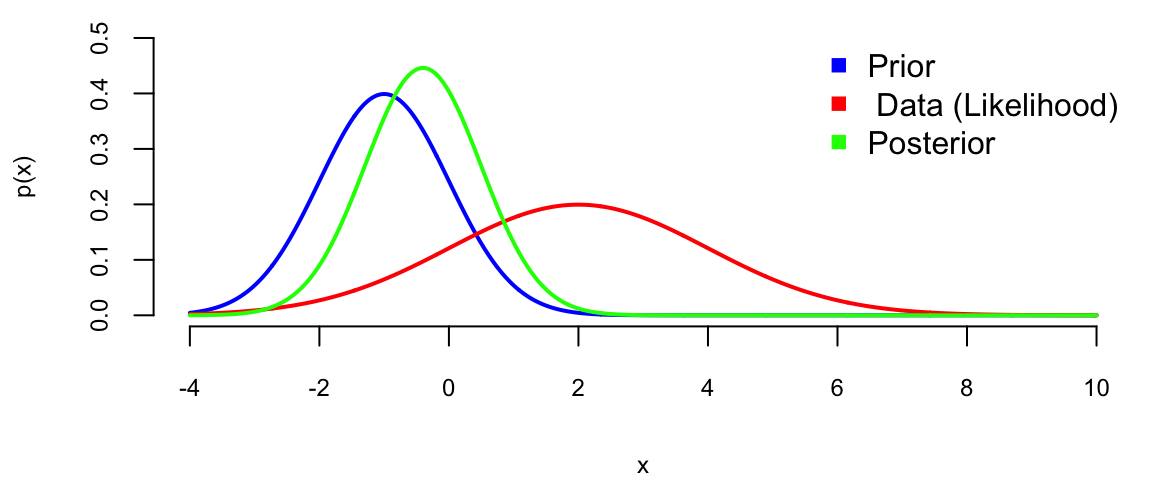
Note, the posterior mean is in between those of prior and likelihood and posterior variance is lower than variance of both prior and likelihood, this is effect of combining information from data and prior!
Consider, another example, when mean \(\mu\) is fixed and variance is a random variable which follows some distribution \(\sigma^2 \sim p(\sigma^2)\). Given an observed sample \(y\), we can update the distribution over variance using the Bayes rule \[ p(\sigma^2 \mid y) = \dfrac{p(y\mid \sigma^2 )p(\sigma^2)}{p(y)}. \] Now, the total probability in the denominator can be calculated as \[ p(y) = \int p(y\mid \sigma^2 )p(\sigma^2) d\sigma^2. \]
In general, this integral cannot be calculated analytically and Bayesian inference relies on numerical approximations. However, for specific choices of the prior distribution \(p(\sigma)\) and likelihood \(p(y\mid \sigma^2 )\), it is possible to analytically calculate the integral and thus, the posterior distribution.
A prior that leads to analytically calculable integral (conjugate prior) for normal likelihood is the inverse Gamma. Thus, if \[ \sigma^2 \mid \alpha,\beta \sim IG(\alpha,\beta) = \dfrac{\beta^{\alpha}}{\Gamma(\alpha)}\sigma^{2(-\alpha-1)}\exp\left(-\dfrac{\beta}{\sigma^2}\right) \] and \[ y \mid \mu,\sigma^2 \sim N(\mu,\sigma^2) \] Then the posterior distribution is another inverse Gamma \(IG(\alpha_{\mathrm{posterior}},\beta_{\mathrm{posterior}})\), with \[ \alpha_{\mathrm{posterior}} = \alpha + 1/2, ~~\beta_{\mathrm{posterior}} = \beta + \dfrac{y-\mu}{2}. \]
Now, the predictive distribution over \(y\) can be calculated by \[ p(y_{new}\mid y) = \int p(y_{new},\sigma^2\mid y)p(\sigma^2\mid y)d\sigma^2. \] Which happens to be a \(t\)-distribution with \(2\alpha_{\mathrm{posterior}}\) degrees of freedom, mean \(\mu\) and variance \(\alpha_{\mathrm{posterior}}/\beta_{\mathrm{posterior}}\).
In the multivriate case, the normal-normal model is \[ \theta \sim N(\mu_0,\Sigma_0), \quad y \mid \theta \sim N(\theta,\Sigma). \] The posterior distribution is \[ \theta \mid y \sim N(\mu_1,\Sigma_1), \] where \[ \Sigma_1 = (\Sigma_0^{-1} + \Sigma^{-1})^{-1}, \quad \mu_1 = \Sigma_1(\Sigma_0^{-1}\mu_0 + \Sigma^{-1}y). \] The predictive distribution is \[ y_{new} \mid y \sim N(\mu_1,\Sigma_1 + \Sigma). \]
Example 4.7 (Satya Nadella: CEO of Microsoft) In 2014, Satya Nadella became the CEO of Microsoft. The stock price of Microsoft has been on a steady rise since then. Suppose that you are a portfolio manager and you are interested in analyzing the returns of Microsoft stock compared to the market.
Suppose you are managing a portfolio with two positions stock of Microsoft (MSFT) and an index fund that follows S&P500 index and tracks overall market performance. We ars interested in estimating the mean returns of the positions in our portfolio. You believe that the returns are normally distributed and are related to each other. You have prior beliefs about these returns, which are also normally distributed. We will use what is called the empirical prior for the mean returns. This is a prior that is based on historical data. The empirical prior is a good choice when you have a lot of historical data and you believe that the future mean returns will be similar to the historical mean returns. We assume the prior for the mean returns is a bivariate normal distribution, let \(\mu_0 = (\mu_{M}, \mu_{S})\) represent the prior mean returns for the stocks. The covariance matrix \(\Sigma_0\) captures your beliefs about the variability and the relationship between these stocks’ returns in the prior. We will use the sample mean and covariance matrix of the historical returns as the prior mean and covariance matrix. The prior covariance matrix is given by \[ \Sigma_0 = \begin{bmatrix} \sigma_{M}^2 & \sigma_{MS} \\ \sigma_{MS} & \sigma_{S}^2 \end{bmatrix}, \] where \(\sigma_{M}^2\) and \(\sigma_{S}^2\) are the sample variances of the historical returns of MSFT and SPY, respectively, and \(\sigma_{MS}\) is the sample covariance of the historical returns of MSFT and SPY. The prior mean is given by \[ \mu_0 = \begin{bmatrix} \mu_{M} \\ \mu_{S} \end{bmatrix}, \] where \(\mu_{M}\) and \(\mu_{S}\) are the sample means of the historical returns of MSFT and SPY, respectively. The likelihood of observing the data, given the mean returns, is also a bivariate normal distribution. The mean of this distribution is the true (but unknown) mean returns \(\mu = [\mu_A, \mu_B]\). The covariance matrix \(\Sigma\) of the likelihood represents the uncertainty in your data. We will use the sample mean and covariance matrix of the observed returns as the likelihood mean and covariance matrix. The likelihood covariance matrix is given by \[ \Sigma = \begin{bmatrix} \sigma_{M}^2 & \sigma_{MS} \\ \sigma_{MS} & \sigma_{S}^2 \end{bmatrix}, \] where \(\sigma_{M}^2\) and \(\sigma_{S}^2\) are the sample variances of the observed returns of MSFT and SPY, respectively, and \(\sigma_{MS}\) is the sample covariance of the observed returns of MSFT and SPY. The likelihood mean is given by \[ \mu = \begin{bmatrix} \mu_{M} \\ \mu_{S} \end{bmatrix}, \] where \(\mu_{M}\) and \(\mu_{S}\) are the sample means of the observed returns of MSFT and SPY, respectively. In a Bayesian framework, you update your beliefs (prior) about the mean returns using the observed data (likelihood). The posterior distribution, which combines your prior beliefs and the new information from the data, is also a bivariate normal distribution. The mean \(\mu_{\text{post}}\) and covariance \(\Sigma_{\text{post}}\) of the posterior are calculated using Bayesian updating formulas, which involve \(\mu_0\), \(\Sigma_0\), \(\mu\), and \(\Sigma\).
We use observed returns prior to Nadella’s becoming CEO as our prior and analyze the returns post 2014. Thus, our observed data includes July 2015 - Dec 2023 period. We assume the likelihood of observing this data, given the mean returns, is also a bivariate normal distribution. The mean of this distribution is the true (but unknown) mean returns. The covariance matrix \(Sigma\) of the likelihood represents the uncertainty in your data and is calculated from the overall observed returns data 2001-2023.
getSymbols(c("MSFT", "SPY"), from = "2001-01-01", to = "2023-12-31") "MSFT" "SPY" s = 3666 # 2015-07-30
prior = 1:s
obs = s:nrow(MSFT) # post covid
# obs = 5476:nrow(MSFT) # 2022-10-06 bull run if 22-23
a = as.numeric(dailyReturn(MSFT))
c = as.numeric(dailyReturn(SPY))
# Prior
mu0 = c(mean(a[prior]), mean(c[prior]))
Sigma0 = cov(data.frame(a=a[prior],c=c[prior]))
# Data
mu = c(mean(a[obs]), mean(c[obs]))
Sigma = cov(data.frame(a=a,c=c))
# Posterior
SigmaPost = solve(solve(Sigma0) + solve(Sigma))
muPost = SigmaPost %*% (solve(Sigma0) %*% mu0 + solve(Sigma) %*% mu)
# Plot
plot(a[obs], c[obs], xlab="MSFT", ylab="SPY", xlim=c(-0.005,0.005), ylim=c(-0.005,0.005), pch=16, cex=0.5)
abline(v=0, h=0, col="grey")
abline(v=mu0[1], h=mu0[2], col="blue",lwd=3) #prior
abline(v=mu[1], h=mu[2], col="red",lwd=3) #data
abline(v=muPost[1], h=muPost[2], col="green",lwd=3) #posterior
legend("bottomright", c("Prior", "Likelihood", "Posterior"), pch=15, col=c("blue", "red", "green"), bty="n")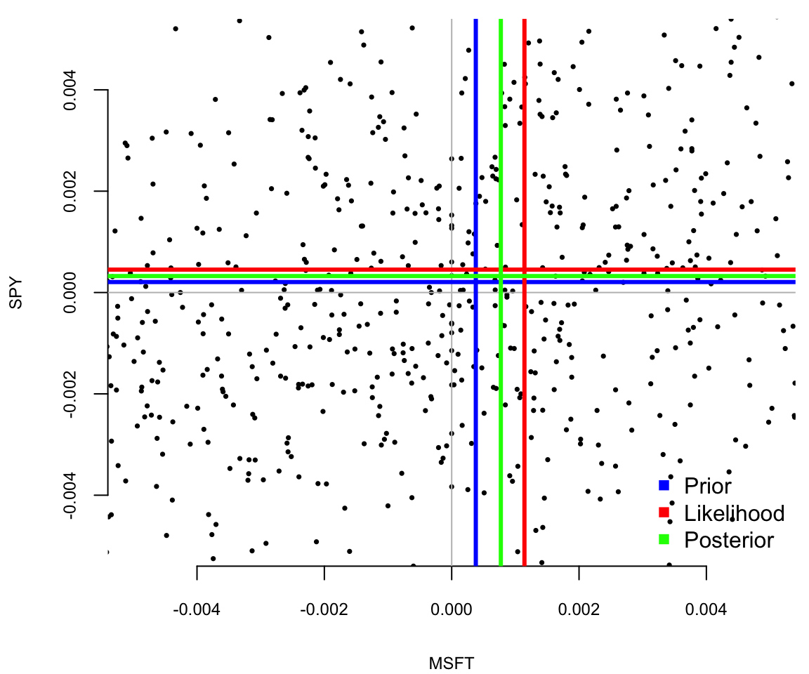
We can see tha posterior mean for SPY is close to the prior mean, while the posterior mean for MSFT is further away. The perofrmance of MSFT was significantly better past 2015 compared to SPY. The posterior mean (green) represents mean reversion value. We can think of it a expected mean return if the perofrmance of MSFT starts reverting to its historical averages.
This model is particularly powerful because it can be extended to more dimensions (more stocks) and can include more complex relationships between the variables. It’s often used in finance, econometrics, and other fields where understanding the joint behavior of multiple normally-distributed variables is important.
Exponential distribution is a continuous distribution that is often used to model waiting times between events. For example, the time between two consecutive arrivals of a Poisson process is exponentially distributed. If the number of events in 1 unit of time has the Poisson distribution with rate parameter \(\lambda\), then the time between events has the exponential distribution with mean \(1/\lambda\). The probability density function (PDF) of an exponential distribution is defined as: \[ f(x;\lambda) = \lambda e^{-\lambda x}, ~ x \geq 0 \] The exponential distribution is defined for \(x \geq 0\), abd \(\lambda\) is the rate parameter, which is the inverse of the mean (or expected value) of the distribution. It must be greater than 0. The exponential distribution is a special case of the Gamma distribution with shape 1 and scale \(1/\lambda\).
The mean and variance are give in terms of the rate parameter \(\lambda\) as
| Exponential Distribution | Parameters |
|---|---|
| Expected value | \(\mu = \E{X} = 1/\lambda\) |
| Variance | \(\sigma^2 = \Var{X} = 1/\lambda^2\) |
Here are some examples of when exponential model provides a good fit
In these examples, the key assumption is that events happen independently and at a constant average rate, which makes the exponential distribution a suitable model.
The Exponential-Gamma model, often used in Bayesian statistics, is a hierarchical model where the exponential distribution’s parameter is itself modeled as following a gamma distribution. This approach is particularly useful in situations where there is uncertainty or variability in the rate parameter of the exponential distribution.
The Exponential-Gamma model assumes that the data follows an exponential distribution (likelihood). As mentioned earlier, the exponential distribution is suitable for modeling the time between events in processes where these events occur independently and at a constant rate. At the next level, the rate parameter \(\lambda\) of the exponential distribution is assumed to follow a gamma distribution. The gamma distribution is a flexible two-parameter family of distributions and can model a wide range of shapes. \[\begin{align*} \lambda &\sim \text{Gamma}(\alpha, \beta) \\ x_i &\sim \text{Exponential}(\lambda) \end{align*}\]
The probability density function of the gamma distribution is given by Equation 4.2 and has two parameters, shape \(\alpha\) and rate \(\beta\). The posterior distribution of the rate parameter \(\lambda\) is given by: \[ p(\lambda\mid x_1, \ldots, x_n) \propto \lambda^{\alpha - 1} e^{-\beta\lambda} \prod_{i=1}^n \lambda e^{-\lambda x_i} = \lambda^{\alpha + n - 1} e^{-(\beta + \sum_{i=1}^n x_i)\lambda} \] which is a gamma distribution with shape parameter \(\alpha + n\) and rate parameter \(\beta + \sum_{i=1}^n x_i\). The posterior mean and variance are given by: \[ \mathbb{E}[\lambda|x_1, \ldots, x_n] = \frac{\alpha + n}{\beta + \sum_{i=1}^n x_i}, \quad \mathrm{Var}[\lambda|x_1, \ldots, x_n] = \frac{\alpha + n}{(\beta + \sum_{i=1}^n x_i)^2}. \] Notice, that \(\sum x_i\) is the sufficient statistic for inference about parameter \(\lambda\)!
Some applicaitons of this model include the following:
In these applications, the Exponential-Gamma model offers a more nuanced approach than using a simple exponential model, as it accounts for the variability in the rate parameter.
Before decideng on a parametric model for a dataset. There are several tools that we use to choose the appropriate model. These include
The two most common tools for exploratory data analysis are Q-Q plot, scatter plots and bar plots/histograms.
A Q-Q plot simply compares the quantiles of your data with the quantiles of a theoretical distribution (like normal, exponential, etc.). Quantile is the fraction (or percent) of points below the given value. That is, the \(i\)-th quantile is the point \(x\) for which \(i\)% of the data lies below \(x\). On a Q-Q plot, if the two data sets come from a population with the same distribution, we should see the points forming a line that’s roughly straight. More precisely, if the two data sets \(x\) and \(y\) come from the same distribution, then the points \((x_{(i)}, y_{(i)})\) should lie roughly on the line \(y = x\). If \(y\) comes from a distribution that’s linear in \(x\), then the points \((x_{(i)}, y_{(i)})\) should lie roughly on a line, but not necessarily on the line \(y = x\).
Example 4.8 (Noraml Q-Q plot) Figure 4.4 shows the normal Q-Q plot for the Data on birth weights of babies born in a Brisbane hospital on December 18, 1997. The data set contains 44 records. A more detailed description of the data set can be found in UsingR manual.
require(UsingR)
qqnorm(babyboom$wt)
qqline(babyboom$wt)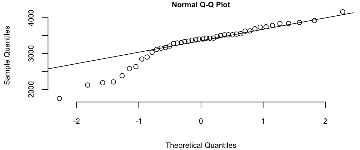
Visually, the answer to answer the question “Are Birth Weights Normally Distributed?” is no. We can see that on the lefrt side of the plot the points are below the line. This indicates that the data is skewed to the left. The data is not normally distributed.
The Q-Q plots look different if we split the data based on the gender
g = babyboom %>% filter(gender=="girl") %>% pull(wt)
b = babyboom %>% filter(gender=="boy")  %>% pull(wt)
qqnorm(g); qqline(g)
qqnorm(b); qqline(b)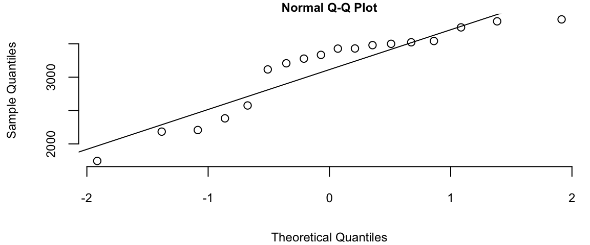
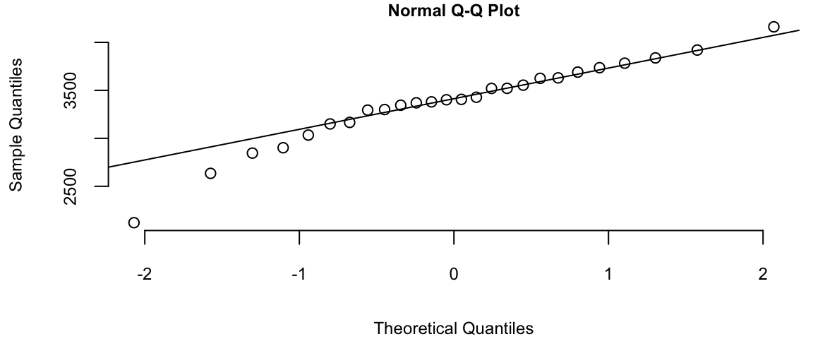
Histogram of baby weights by gender
How about the times in hours between births of babies?
hr = ceiling(babyboom$running.time/60)
BirthsByHour = tabulate(hr)
# Number of hours with 0, 1, 2, 3, 4 births
ObservedCounts = table(BirthsByHour)
# Average number of births per hour
BirthRate=sum(BirthsByHour)/24
# Expected counts for Poisson distribution
ExpectedCounts=dpois(0:4,BirthRate)*24
# bind into matrix for plotting
ObsExp <- rbind(ObservedCounts,ExpectedCounts)
barplot(ObsExp,names=0:4, beside=TRUE,legend=c("Observed","Expected"))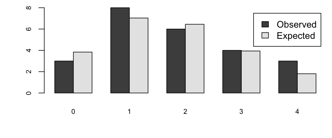
What about the Q-Q plot?
# birth intervals
birthinterval=diff(babyboom$running.time)
 # quantiles of standard exponential distribution (rate=1)
exponential.quantiles = qexp(ppoints(43))
qqplot(exponential.quantiles, birthinterval)
lmb=mean(birthinterval)
lines(exponential.quantiles,exponential.quantiles*lmb) # Overlay a line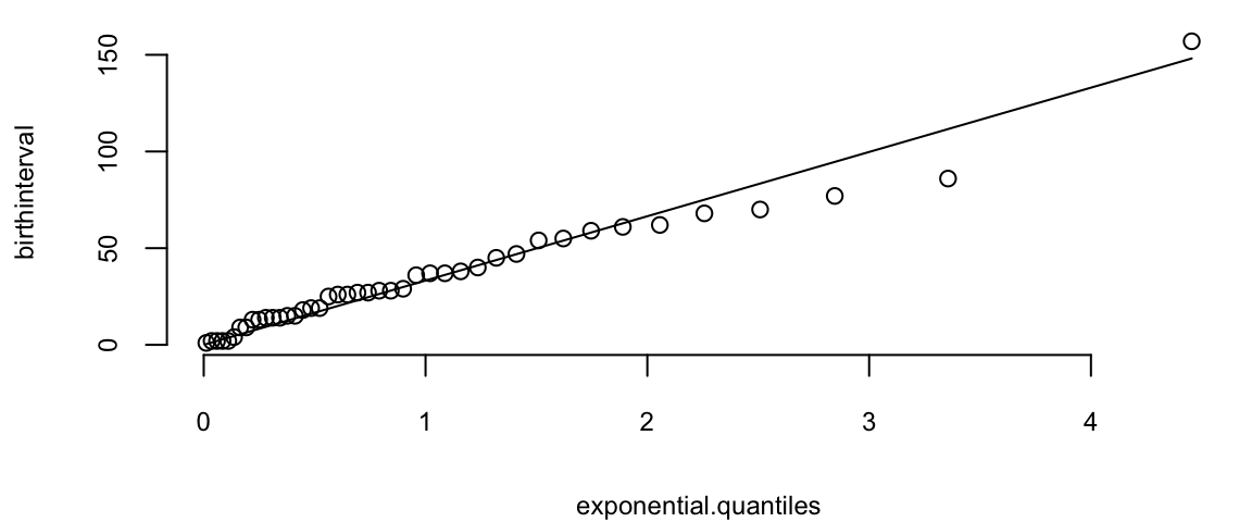
Here
ppoints function computes the sequence of probability pointsqexp function computes the quantiles of the exponential distributiondiff function computes the difference between consecutive elements of a vectorTable 4.1 summarizes the conjugate prior distributions for common likelihoods. Thus far, we’ve conidered the Normal-Normal model with both known and unknown variance as well as Poisson-Gamma and Beta Binomial. The other pairs are left as an exercise.
| Likelihood Distribution | Conjugate Prior Distribution | Prior Parameters | Likelihood Parameters | Posterior Parameters |
|---|---|---|---|---|
| Normal (known \(\sigma^2\)) | Normal | \(\mu_0, \sigma^2_0\) | \(\mu, \sigma^2\) | \(\frac{\sigma^2_0 \cdot \mu + \sigma^2 \cdot \mu_0}{\sigma^2 + \sigma^2_0}, \frac{1}{\frac{1}{\sigma^2_0} + \frac{1}{\sigma^2}}\) |
| Normal (unknown \(\sigma^2\)) | Normal-Inverse Gamma | \(\mu_0, \lambda_0, \alpha_0, \beta_0\) | \(\mu, \sigma^2\) | \(\mu_{n}, \lambda_{n}, \alpha_{n}, \beta_{n}\) |
| Binomial | Beta | \(\alpha, \beta\) | \(n, x\) | \(\alpha + x, \beta + n - x\) |
| Poisson | Gamma | \(\alpha, \beta\) | \(\lambda\) | \(\alpha + \sum x_i, \beta + n\) |
| Exponential | Gamma | \(\alpha, \beta\) | \(\lambda\) | \(\alpha + n, \beta + \sum x_i\) |
| Multinomial | Dirichlet | \(\boldsymbol{\alpha}\) | \(\boldsymbol{x}\) | \(\boldsymbol{\alpha} + \boldsymbol{x}\) |
| Normal (unknown mean, unknown variance) | Normal-Inverse-Wishart | \(\mu_0, \kappa_0, \nu_0, \Psi_0\) | \(\mu, \Sigma\) | Updated \(\mu_{n}, \kappa_{n}, \nu_{n}, \Psi_{n}\) |
These conjugate relationships simplify Bayesian calculations by ensuring that the posterior distributions are in the same family as the priors.
Yet another fundamental concept that is useful for probabilistic reasoning is stochastic priocess. An instance of a process is a function \(Y:~ U \rightarrow S\) from domain of index set \(U\) into another set of process values \(S\), called state-space. The state-space of a stochastic process is the set of all possible states that the process can be in. Each state in the state-space represents a possible outcome or condition of the system being modeled. The process then is the distribution over the space of functions from \(U\) to \(S\). The term process is used because the function \(Y\) is often thought of as a time-varying quantity, and the index set \(U\) is often interpreted as time. However, the index set can be any set, and the process can be a random function of any other variable. Both index set and state-space can be discrete or continuous. For example, descrete time index can represent days or rounds and continoius time index is a point on a time line. The state-space can be discrete (composed of distinct states, like the number of customers in a store) or continuous (such as the price of a stock). The state-space can be one-dimensional (only one aspect of the system is modeled) or multi-dimensional (multiple aspects are modeled simultaneously).
Here are some widely used stochastic processes:
In contexts like agricultural field trials, the domain for analyzing yield is commonly referred to as the collection of plots. This term is broadly suitable for practical field purposes but is mathematically interpreted as the collection of planar Borel subsets across various growing seasons. In a basic clinical trial for a COVID-19 vaccine, like the AstraZeneca trial in 2021, the domain is typically referred to as the group of patients. This implies the inclusion of all eligible patients, regardless of whether they were actually recruited and observed in the trial. In research on speciation or sexual compatibility in fruit flies, the domain is defined as the set of male-female pairs, encompassing all potential pairs with the desired genetic traits. For a competition experiment, such as a chess or tennis tournament, the domain is described as the set of ordered pairs of participants, which includes all possible pairings, not just those who actually competed against each other at events like US Open in 2024.
In data analysis, both experimental and observational data can exhibit variability. This variability is often modeled using probability distributions. These distributions can either represent simple processes with independent elements (then we are back to i.i.d case) or more complex stochastic processes that display dependencies, whether they be serial, spatial, or of other types. Essentially, this modeling approach helps in understanding and predicting data behavior under various conditions. The early sections of Davison (2003) work offer an insightful primer on how to develop and apply these stochastic models across various fields. This introduction is particularly useful for grasping the fundamental concepts and practical applications of these models.
Brownian Motion, named after botanist Robert Brown, is a fundamental concept in the theory of stochastic processes. It describes the random motion of particles suspended in a fluid (liquid or gas), as they are bombarded by the fast-moving molecules in the fluid.
The mathematical model of Brownian Motion, \(B(t)\), where \(t\) represents time. For \(s < t\), the increment \(B(t) - B(s)\) is normally distributed with mean 0 and variance \(t - s\), i.e., \(B(t) - B(s) \sim N(0, t-s)\). The process \(B(t)\) is continuous, but nowhere differentiable. Figure 4.5 below shows tree sample paths of Brownian Motion.
# Brownian Motion
t = seq(0, 1, 0.001)
plot(t, cumsum(rnorm(1001, 0, sqrt(0.001))), type="l", xlab="t", ylab="B(t)", lwd=2)
lines(t, cumsum(rnorm(1001, 0, sqrt(0.001))), lwd=2, col=2)
lines(t, cumsum(rnorm(1001, 0, sqrt(0.001))),lwd=2, col=3)
legend("topright", c("Path 1", "Path 2", "Path 3"), pch=15, col=c(1, 2, 3), bty="n")
Thus, for any times \(0 \leq t_1 < t_2 < ... < t_n\), the random variables \(B(t_2) - B(t_1)\), \(B(t_3) - B(t_2)\), …, \(B(t_n) - B(t_{n-1})\) are independent and the function \(t \mapsto B(t)\) is continuous almost surely.
Some properties of Brownian Motion are:
Scale Invariance: If \(B(t)\) is a Brownian motion, then for any \(a > 0\), the process \(aB(t/a^2)\) is also a Brownian motion.
Time Inversion: If \(B(t)\) is a Brownian motion, then \(tB(1/t)\) is also a Brownian motion for \(t > 0\).
Fractal Nature: Brownian motion paths are nowhere differentiable but continuous everywhere, reflecting a fractal-like nature.
Although it was originally developed to model the random motion of particles in fluids, Brownian Motion has found applications in many other fields, including finance (Black-Scholes model for option pricing, assumes movements in stock prices follow Brownian Motion), biology (movement of biomolecules within cells), environmental science (diffusion processes, like the spread of pollutants in the air or water), and mathematics (stochastic calculus and differential equations).
Example 4.9 (Brownian Motion for Sport Scores) A Model for Sports Scores
In order to define the implied volatility of a sports game we begin with
a distributional model for the evolution of the outcome in a sports game which we develop from Stern (1994). The model specifies the distribution of the lead of team A over team B, \(X(t)\) for any \(t\) as a Brownian motion process. If \(B(t)\) denotes a standard Brownian motion with distributional property \(B(t) \sim N(0,t)\) and we incorporate drift, \(\mu\), and volatility, \(\sigma\), terms, then the evolution of the outcome \(X(t)\) that is given by: \[
X(t)=\mu t + \sigma B(t) \sim N( \mu t , \sigma^2 t).
\] This distribution of the game outcome is similar to the Black-Scholes model of the distribution of a stock price.
This specification results in several useful measures (or, this specification results in closed-form solutions for a number of measures of interest). The distribution of the final score follows a normal distribution, \(X(1)\sim N(\mu, \sigma^2)\). We can calculate the probability of team A winning, denoted \(p=\mathbb{P}(X(1)>0)\), from the spread and probability distribution. Given the normality assumption, \(X(1) \sim N(\mu, \sigma^2)\), we have \[ p = \mathbb{P}(X(1)>0) = \Phi \left ( \frac{\mu}{\sigma} \right ) \] where \(\Phi\) is the standard normal cdf. Table 1 uses \(\Phi\) to convert team A’s advantage \(\mu\) to a probability scale using the information ratio \(\mu/\sigma\).
| \(\mu/\sigma\) | 0 | 0.25 | 0.5 | 0.75 | 1 | 1.25 | 1.5 | 2 |
|---|---|---|---|---|---|---|---|---|
| \(p=\Phi(\mu/\sigma)\) | 0.5 | 0.60 | 0.69 | 0.77 | 0.84 | 0.89 | 0.93 | 0.977 |
If teams are evenly matched and \(\mu/\sigma =0\) then \(p=0.5\). Table 1 provides a list of probabilities as a function of \(\mu/\sigma\). For example, if the point spread \(\mu=-4\) and volatility is \(\sigma=10.6\), then the team has a \(\mu/\sigma = -4/10.6 = - 0.38\) volatility point disadvantage. The probability of winning is \(\Phi(-0.38) = 0.353 < 0.5\). A common scenario is that team A has an edge equal to half a volatility, so that \(\mu/\sigma =0.5\) and then \(p= 0.69\).
Of particular interest here are conditional probability assessments made as the game progresses. For example, suppose that the current lead at time \(t\) is \(l\) points and so \(X(t) = l\). The model can then be used to update your assessment of the distribution of the final score with the conditional distribution $ (X(1) | X(t)=l )$. To see this, we can re-write the distribution of \(X(1)\) given \(X(t)\) by noting that \(X(1) = X(t)+ X(1) - X(t)\). Using the formula above and substituting \(t\) for \(1\) where appropriate and noting that \(X(t) = l\) by assumption, this simplifies to \[ X(1)= l + \mu(1- t) + \sigma (B(1) - B(t)). \] Here \(B(1) - B(t) \stackrel{D}{=} B(1-t)\) which is independent of \(X(t)\) with distribution \(N(0,1-t)\). The mean and variance of \(X(1)|X(t)=l\) decay to zero as \(t \rightarrow 1\) and the outcome becomes certain at the realised value of \(X(1)\). We leave open the possibility of a tied game and overtime to determine the outcome.
To determine this conditional distribution, we note that there are \(1-t\) time units left together with a drift \(\mu\) and as shown above in this case the uncertainty can be modeled as which is Therefore, we can write the distribution of the final outcome after \(t\) periods with a current lead of \(l\) for team A as the conditional distribution: \[ ( X(1) | X(t)=l) = (X(1)-X(t)) + l \sim N( l + \mu(1 - t) , \sigma^2 (1 - t) ) \] From the conditional distribution \((X(1) | X(t)=l) \sim N(l+\mu(1-t), \sigma^2 (1-t))\), we can calculate the conditional probability of winning as the game evolves. The probability of team A winning at time \(t\) given a current lead of \(l\) point is: \[ p_t = P ( X(1) > 0 | X(t) = l) = \Phi \left ( \frac{ l + \mu ( 1 - t) }{ \sigma \sqrt{ ( 1-t) } } \right ) \]
Figure 4.6 A and B illustrate our methodology with an example. Suppose we are analyzing data for a Superbowl game between teams A and B with team A favored. Figure A presents the information available at the beginning of game from the perspective of the undergod team B. If the initial point spread–or the markets’ expectaion of the expected outcome–is \(-4\) and the volatility is \(10.6\)–assumed given for the moment (more on this below)–then the probability that the underdog team wins is \(p = \Phi ( \mu /\sigma ) = \Phi ( - 4/ 10.6) = 35.3\)%. This result relies on our assumption of a normal outcome distribution on the outcome as previously explained. Another way of saying this is \(\mathbb{P}(X(1)>0)=0.353\) for an outcome distribution \(X(1) \sim N(-4, 10.6^2)\). Figure A illustrates this with the shaded red area under the curve.
Figure 4.6 B illustrates the information and potential outcomes at half-time. Here we show the evolution of the actual score until half time as the solid black line. From half-time onwards we simulate a set of possible Monte Carlo paths to the end of the game. %Specifically, we discretise the model with time interval \(\Delta =1/200\) %and simulate possible outcomes given the score at half time. The volatility plays a key role in turning the point spread into a probability of winning as the greater the volatility of the distribution of the outcome, \(X(1)\), the greater the range of outcomes projected in the Monte Carlo simulation. Essentially the volatility provides a scale which calibrates the advantage implied by a given point spread.
We can use this relationship to determine how volatility decays over the course of the game. The conditional distribution of the outcome given the score at time \(t\), is \((X(1)|X(t)=l)\) with a variance of \(\sigma^2(1-t)\) and volatility of \(\sigma \sqrt{1-t}\). The volatility is a decreasing function of \(t\), illustrating that the volatility dissipates over the course of a game. For example, if there is an initial volatility of \(\sigma = 10.6\), then at half-time when \(t=\frac{1}{2}\), the volatility is \(10.6 / \sqrt{2} = 7.5\) volatility points left. Table 2, below, illustrates this relationship for additional points over the game.
| \(t\) | 0 | \(\frac{1}{4}\) | \(\frac{1}{2}\) | \(\frac{3}{4}\) | 1 |
|---|---|---|---|---|---|
| \(\sigma \sqrt{1-t}\) | 10.6 | 9.18 | 7.50 | 5.3 | 0 |
To provide insight into the final outcome given the current score, Tables 1 and 2 can be combined to measure the current outcome, \(l\), in terms of standard deviations of the outcome.
For example, suppose that you have Team B, an underdog, so from their perspective \(\mu = -4\) and at half-time team B has a lead of 15, \(l= 15\). Team B’s expected outcome as presented earlier is \(l + \mu (1-t)\) or \(15 - 4 \times \frac{1}{2} = 13\). If initial volatility is \(\sigma = 10.60\) then the remaining volatility at half-time is \(10.6/\sqrt{2} = 7.50\) and team B’s expected outcome of \(13\) in terms of standard deviations is \(13/7.5 = 1.73\). Thus team B’s expected outcome is at the 99th percentile of the distribution, \(\Phi ( 1.73 ) = 0.96\), implying a 96% chance of winning.
Implied Volatility
The previous discussion assumed that the variance (or volatility) parameter \(\sigma\) was a known constant. We return to this important quantity now.
We are now in a position to define the implied volatility implicit in the two betting lines that are available. Given our model, we will use the money-line odds to provide a market assessment of the probability of winning, \(p\), and the point spread to assess the expected margin of victory, \(\mu\). The money line odds are shown for each team A and B and provide information on the payoff from a bet on the team winning. As shown in the example in section 3, this calculation will also typically require an adjustment for the bookmaker’s spread. With these we can infer the implied volatility, \(\sigma_{IV}\), by solving \[
\sigma_{IV}: \; \; \; \; \; p = \Phi \left ( \frac{\mu}{\sigma_{IV}} \right ) \; \; \text{ which \; gives} \; \;
\sigma_{IV} = \frac{ \mu }{ \Phi^{-1} ( p ) } \; .
\] Here \(\Phi^{-1}(p)\) denotes the standard normal quantile function such that the area under the standard normal curve to the left of \(\Phi^{-1}(p)\) is equal to \(p\). In our example we calculate this using the qnorm in R. Note that when \(\mu =0\) and \(p= \frac{1}{2}\) there’s no market information about the volatility as \(\mu / \Phi^{-1} (p)\) is undefined. This is the special case where the teams are seen as evenly matched- the expected outcome has a zero point spread and there is an equal probability that either team wins.
Time Varying Implied Volatility
Up to this point the volatility rate has been assumed constant through the course of the game, i.e., that the same value of \(\sigma\) is relevant. The amount of volatility remaining in the game is not constant but the basic underlying parameters has been assumed constant. This need not be true and more importantly the betting markets may provide some information about the best estimate of the volatility parameter at a given point of time. This is important because time-varying volatility provides an interpretable quantity that can allow one to assess the value of a betting opportunity.
With the advent of on-line betting there is a virtually continuous traded contract available to assesses implied expectations of the probability of team A winning at any time \(t\). The additional information available from the continuous contract allows for further update of the implied conditional volatility. We assume that the online betting market gives us a current assessment of \(p_t\), that is the current probability that team A will win. We will then solve for \(\sigma^2\) and in turn define resulting time-varying volatility, as \(\sigma_{IV,t}\), using the resulting equation to solve for \(\sigma_{IV,t}\) with \[ p_t = \Phi \left ( \frac{ l + \mu(1-t) }{\sigma_{IV,t} \sqrt{1-t}} \right ) \; \text{ which \; gives} \; \; \sigma_{IV,t} = \frac{ l + \mu ( 1-t ) }{ \Phi^{-1} ( p_t ) \sqrt{1-t}} \] We will use our methodology to find evidence of time-varying volatility in the SuperBowl XLVII probabilities.
Super Bowl XLVII: Ravens vs San Francisco 49ers
Super Bowl XLVII was held at the Superdome in New Orleans on February 3, 2013 and featured the San Francisco 49ers against the Baltimore Ravens. Going into Super Bowl XLVII the San Francisco 49ers were favorites to win which was not surprising following their impressive season. It was a fairly bizarre Super Bowl with a \(34\) minute power outage affecting the game by ultimately an exciting finish with the Ravens causing an upset victory \(34-31\). We will build our model from the viewpoint of the Ravens. Hence \(X(t)\) will correspond to the Raven’s score minus the San Francisco 49ers. Table 3 provides the score at the end of each quarter.
| \(t\) | 0 | \(\frac{1}{4}\) | \(\frac{1}{2}\) | \(\frac{3}{4}\) | 1 |
|---|---|---|---|---|---|
| Ravens | 0 | 7 | 21 | 28 | 34 |
| 49ers | 0 | 3 | 6 | 23 | 31 |
| \(X(t)\) | 0 | 4 | 15 | 5 | 3 |
To determine the parameters of our model we first use the point spread which was set at the Ravens being a four point underdog, i.e. \(\mu=-4\). This sets the mean of our outcome, \(X(1)\), as \[ \mu = \mathbb{E} \left (X(1) \right )=-4 . \] In reality, it was an exciting game with the Ravens upsetting the 49ers by \(34-31\). Hence, the realised outcome is \(X(1)= 34-31=3\) with the point spread being beaten by \(7\) points or the equivalent of a touchdown.
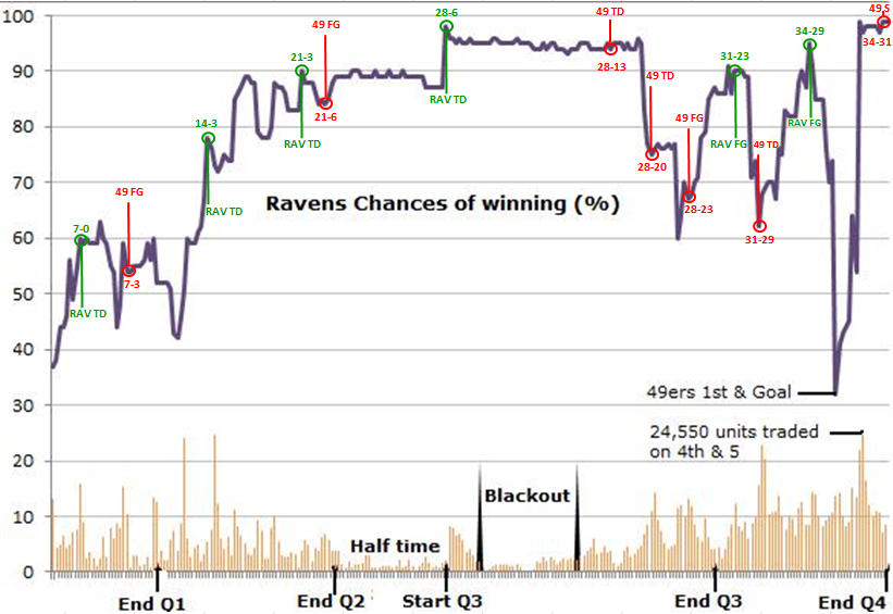
To determine the markets’ assessment of the probability that the Ravens would win at the being of the game we use the money-line odds. These odds were quoted as San Francisco \(-175\) and Baltimore Ravens \(+155\). This implies that a bettor would have to place $175 to win $100 on the 49ers and a bet of $100 on the Ravens would lead to a win of $155. We can convert both of these money-lines to implied probabilities of the each team winning, by the equations \[ p_{SF} = \frac{175}{100+175} = 0.686 \; \; \text{ and} \; \; p_{Ravens} = \frac{100}{100+155} = 0.392 \] The probability sum to one plus the market vig: \[ p_{SF} + p_{Ravens} = 0.686+0.392 = 1.078 \] namely a \(7.8\)% edge for the bookmakers. Put differently, if bettors place money proportionally across both teams then the bookies will make \(7.8\)% of the total staked no matter what happens to the outocme of the game. To account for this edge in our model, we use the mid-point of the spread to determine \(p\) implying that \[ p = \frac{1}{2} p_{Ravens} + \frac{1}{2} (1 - p_{SF} ) = 0.353 \] From the Ravens perspective we have \(p = \mathbb{P}(X(1)>0) =0.353\).
Figure 4.7 shows the evolution of the markets conditional probability of winning \(p_t\) for the Ravens. The data are from the online betting website TradeSports.com. Starting at \(p=0.353\) we see how dramatically the markets assessment of the Ravens winning can fluctuate. (NGP: This is really confusing. We need to say a bit more about what we did here. How do you get these probabilities. Key point is what are you assuming about sigma given the abaove discussion.) Given their commanding lead at half time, the probability has as high as \(0.90\). At the end of the four quarter when the 49ers nearly went into the lead with a touchdown, at one point the probability had dropped to \(30\)%.
Our main question of interest is then: What implied volatility is consistent with market expectations?
To calculate the implied volatility of the Superbowl we substitute the pair \((\mu,p)\) into our definition and solve for \(\sigma_{IV}\). We obtain \[ \sigma_{IV} = \frac{\mu}{\Phi^{-1}(p)} = \frac{-4}{-0.377} = 10.60 \] where we have used \(\Phi^{-1} ( p) = qnorm(0.353) = -0.377\). So on a volatility scale the \(4\) point advantage assessed for the 49ers is under a \(\frac{1}{2} \sigma\) favorite. From Table 2, this is consistent with a win probability of \(p=\Phi(\frac{1}{2})=0.69\). Another feature is that a \(\sigma=10.6\) is historically low, as a typical volatility of an NFL game is \(14\) (see Stern, 1991). However, the more competitive the game one might expect a lower volatility. In reality, the outcome \(X(1)=3\) was withing one standard deviation of the model which had an expectation of \(\mu=-4\) and volatility of \(\sigma= 10.6\). Another question of interest is
What’s the probability of the Ravens winning given their lead at half time?
To illustrate the dynamic nature of the odds and to infer a time-varying implied volatility we ask the question,
At half time the Ravens where leading \(21\) to \(6\). This gives us \(X(\frac{1}{2})=21-6=15\). From the online betting market we also have traded contracts on TradeSports.com that yield a current probability of \(p_{\frac{1}{2}} = 0.90\). Now we can ask
An alternative view is to assume that the market assesses time varying volatility and the prices fully reflect the underlying probability. Here we ask the question
What’s the implied volatility for the second half of the game?
We now have an implied volatility \[
\sigma_{IV,t=\frac{1}{2}} = \frac{ l + \mu ( 1-t ) }{ \Phi^{-1} ( p_t ) \sqrt{1-t}} = \frac{15-2}{ \Phi^{-1}(0.9) / \sqrt{2} } = 14
\] where qnorm(0.9)=1.28. Notice that \(14> 10.6\), our assessment of the implied volatility at the beginning of the game.
What’s a valid betting strategy?
An alternative approach is to assume that the initial moneyline and point spread set the volatility and this stays constant throughout the game. This market is much larger than the online market and this is a reasonable assumption unless there has been material information as the game progresses such as a key injury.
Hence the market was expected a more typical volatility in the second half. If a bettor believed that there was no reason that \(\sigma\) had changed from the initial \(10.6\) then their assessment of the Ravens win probability, under this models, would have been \(\Phi \left ( 13/ (10.6/\sqrt{2}) \right ) = 0.96\) and the \(0.90\) market rate would have been thought of as a betting opportunity.
The Kelly criterion (Kelly,1956) yields the betting rate \[ \omega = p - \frac{q}{0} = 0.96 - \frac{0.1}{1/9} = 0.06 \] that is, \(6\)% of capital. A more realistic strategy is to use the fractional Kelly criterion whcih scales by a risk aversion parameter, \(\gamma\). For example, in this case if \(\gamma =3\), we would bet \(0.06/3=0.01\), or \(2\)% of our capital on this betting opportunity.
Finally, odds changes can be dramatic at the end of the fourth quarter and this Super Bowl was no exception. With the score at \(34-29\), with \(x\) minutes to go, the 49ers were at \(1\)st and goal. in the minutes before this, the probability of the Ravens winning had dropped precipitously from over \(90\)% to \(30\)%, see Figure 4.7. On San Francisco’s final offensive play of the game, Kaepernick threw a pass on fourth down to Michael Crabtree, but Ravens cornerback Jimmy Smith appeared to hold the wide receiver during the incompletion, No call was given and the final result was a Ravens win.
A Gaussian Process (GP) is a collection of random variables, any finite number of which have a joint Gaussian distribution. It’s a powerful tool for modeling and predicting in various fields, particularly useful for regression and classification tasks in machine learning.
A Gaussian Process is completely specified by its mean function \(m(x)\) and covariance function \(k(x, x')\), where \(x\) and \(x'\) are points in the input space. The mean function defines the average value of the function at point \(x\), and the covariance function, also known as the kernel, defines the extent to which the values of the function at two points \(x\) and \(x'\) are correlated.
A Gaussian Process is denoted as: \[ f(x) \sim \mathcal{GP}(m(x), k(x, x')) \]
Flexibility in Modeling Correlations: Through the choice of the kernel function, GPs can model a wide range of correlations between the data points.
Non-Parametric Nature: GPs are considered non-parametric, which means they can model functions of arbitrary complexity.
Incorporation of Prior Knowledge: The mean and covariance functions can incorporate prior knowledge about the behavior of the function being modeled.
Machine Learning: Used for regression tasks, GPs can predict the value of a function at new points, taking into account the uncertainty of the prediction.
Spatial Data Analysis: GPs are effective in modeling spatial data, where the correlation between data points is often related to their physical distance.
Time Series Forecasting: They can be used to model and predict time series data, where the kernel function can capture temporal correlations.
Environmental Modeling: In environmental science, GPs are used for modeling and predicting various phenomena, such as temperature or pollution levels, over geographical areas.
Robotics: For path planning and mapping in uncertain environments, where the robot uses GP to model and predict the terrain.
In summary, Gaussian Processes provide a robust and flexible framework for modeling and predicting in situations where uncertainty and correlation among data points play a critical role. Their versatility and powerful predictive capabilities make them a popular choice in various scientific and engineering disciplines.
Gaussian Processes (GPs) are a collection of random variables, any finite number of which have a joint Gaussian distribution. They are used in machine learning for regression and classification tasks. A GP is a stochastic process where any point in the domain is assigned a random variable. The GP is fully specified by its mean function and covariance function. The mean function is the expected value of the random variable at each point in the domain. The covariance function specifies the covariance between the random variables at any two points in the domain. The covariance function is also called the kernel function. The kernel function is a measure of similarity between two points in the domain. The covariance between two points is higher if they are similar, and lower if they are dissimilar. The kernel function is often chosen to be a function of the distance between the two points. The most commonly used kernel function is the squared exponential kernel, which is a function of the squared distance between the two points. The squared exponential kernel is also called the radial basis function (RBF) kernel. The squared exponential kernel is given by: \[ k(x, x') = \sigma^2 \exp\left(-\frac{(x - x')^2}{2l^2}\right) \] where \(\sigma^2\) is the variance parameter and \(l\) is the length scale parameter. The variance parameter controls the vertical variation of the function, and the length scale parameter controls the horizontal variation. The length scale parameter determines how far apart two points must be to be considered dissimilar. The larger the length scale, the smoother the function. The length scale parameter is also called the bandwidth parameter. The squared exponential kernel is a stationary kernel, which means that it is a function of the distance between the two points and not the actual values of the points. The squared exponential kernel is infinitely differentiable, which means that the GP is a very smooth function. The squared exponential kernel is also called the radial basis function (RBF) kernel.