9  Unreasonable Effectiveness of Data

Telescopes played a crucial role in the advancement of observational astronomy, enabling scientists like Carl Friedrich Gauss, Pierre-Simon Laplace, and Siméon Denis Poisson to collect large amounts of astronomical data. The availability of this data, in turn, led to the development of new data analysis techniques and statistical methods during the late 18th and early 19th centuries.

The availability of data from telescopic observations during the late 18th and early 19th centuries played a pivotal role in the development of new data analysis techniques by Gauss, Laplace, and Poisson. These techniques, such as the method of least squares and the Poisson distribution, were not only crucial for astronomy but also had broader applications in statistics and mathematical modeling. The integration of observational data and statistical methods marked a significant shift in the scientific approach, enabling more rigorous analysis and interpretation of astronomical phenomena.

Back in the 18th and 19th century data collection was often limited to manual measurements or observations, and the amount of available data was typically much smaller compared to the massive datasets encountered in modern data science. Scientists like Gauss and Poisson often conducted carefully designed experiments, collected their own data, and performed manual calculations without the aid of computers or advanced statistical software. The focus of their work was often on theoretical developments in mathematics, physics and astronomy, and the data was used to test and validate their theories. Let’s consider one of those studies from early 18th century.

Example 9.1 (Boscovich and Shape of Earth) The 18th century witnessed heated debates surrounding the Earth’s precise shape. While the oblate spheroid model – flattened poles and bulging equator – held sway, inconsistencies in measurements across diverse regions fueled uncertainty about its exact dimensions. The French, based on extensive survey work by Cassini, maintained the prolate view while the English, based on gravitational theory of Newton (1687), maintained the oblate view.

The determination of the exact figure of the earth would require very accurate measurements of the length of a degree along a single meridian. The final answer to this debate was given by Roger Boscovich (1711–1787) who used geodetic surveying principles and in collaboration with English Jesuit Christopher Maire, in 1755, they embarked on a bold project: measuring a meridian arc spanning a degree of latitude between Rome and Rimini. He employed ingenious techniques to achieve remarkable accuracy for his era, minimizing errors and ensuring the reliability of his data. In 1755 they published “De litteraria expeditione per pontificiam ditionem” (On the Scientific Expedition through the Papal States) that contained results of their survey and its analysis. For more details about the work of Boscovich, see Altić (2013). Stigler (1981) gives an exhaustive introduction to the history of regression.

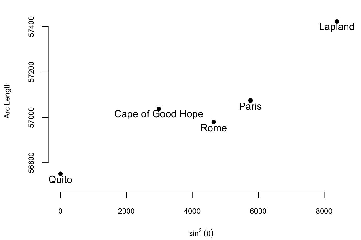
The data on meridian arcs used by Boscovich was crucial in determining the shape and size of the Earth. He combined data from five locations:

Code

d=read.csv("../../data/boscovich.csv")
knitr::kable(d, digits = 8)

Location	Latitude	ArcLength	sin2Latitude
Quito	0	56751	0
Cape of Good Hope	33	57037	2987
Rome	43	56979	4648
Paris	49	57074	5762
Lapland	66	57422	8386

Code

plot(d$sin2Latitude,d$ArcLength, ylab="Arc Length", xlab=expression(sin^2~(theta)), pch=16,ylim=c(56700,57450), xlim=c(-30,8590))
text(d$sin2Latitude,d$ArcLength-25, labels=d$Location)

The arc length is measured in toises. A toise is a pre-metric unit of length approximately equal to 6.39 feet. 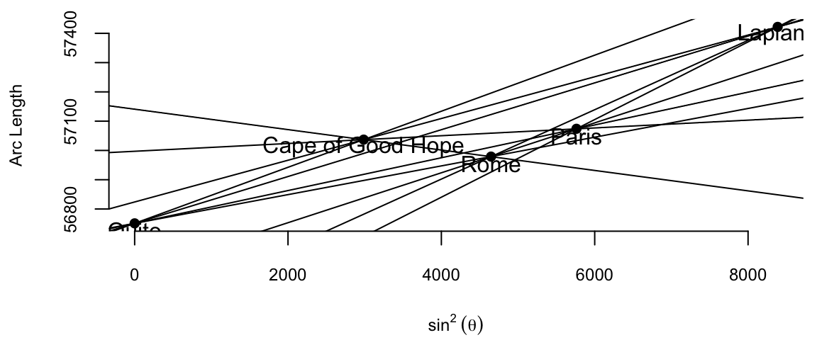It is clear from the table and from the table and from the plot that the the arc length goes up as the latitude increases and the relationship between the arc length and the sine squared of the latitude is approximately linear and the relationship is \[ \text{Arc Length} = \beta_0 + \beta_1 \sin^2 \theta \] where \(\theta\) is the latitude. Here \(\beta_0\) is the length of a degree of arc at the equator, and \(\beta_1\) is how much longer a degree of arc is at the pole. The question that Boscovich asked is how can we combine those five data points to estimate the parameters \(\beta_0\) and \(\beta_1\)? His first attempt to answer this question involved calculating ten slopes for each pair of points and then averaging them. The table below shows the ten slopes.

Code

d = read.csv("../../data/boscovich.csv")
sl = matrix(NA,5,5)
for (i in 1:5) {
    for(j in 1:(i-1)) {
        dx = d$sin2Latitude[i] - d$sin2Latitude[j]
        dy = d$ArcLength[i] - d$ArcLength[j]
        sl[i,j]=dy/dx
    }
}
rownames(sl) = d$Location
colnames(sl) = d$Location
options(knitr.kable.NA = '')
knitr::kable(sl, digits = 4)

Ten slopes for each pair of the five cities from the Boscovich data

	Quito	Cape of Good Hope	Rome	Paris	Lapland
Quito
Cape of Good Hope	0.096
Rome	0.049	-0.035
Paris	0.056	0.013	0.085
Lapland	0.080	0.071	0.118	0.13

Ten slopes for each pair of the five cities from the Boscovich data

Code

plot(d$sin2Latitude,d$ArcLength, ylab="Arc Length", xlab=expression(sin^2~(theta)), pch=16)
text(d$sin2Latitude,d$ArcLength-25, labels=d$Location)
for (i in 1:4){
  for (j in (i+1):5){
    slope = (d$ArcLength[i] - d$ArcLength[j])/(d$sin2Latitude[i] - d$sin2Latitude[j])
    intercept = d$ArcLength[i] - slope*d$sin2Latitude[i]
    abline(a=intercept, b=slope)
  }
}

Ten slopes for each pair of the five cities from the Boscovich data

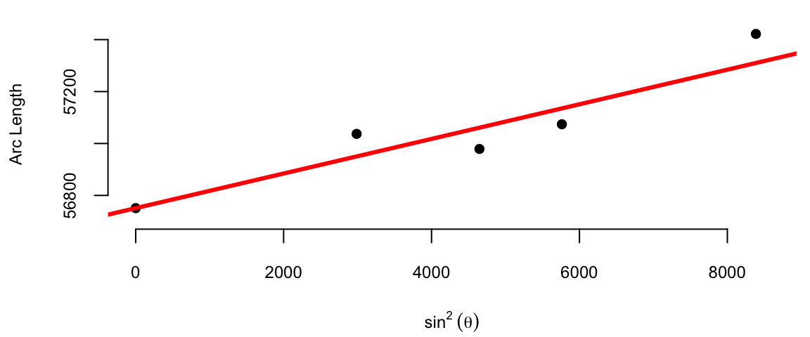
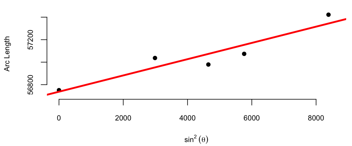
The average of the ten slopes is 0.0667. Notice the slope between Cape of Good Hope and Rome is negative. This is due to the measurement error. Boscovich then calculated an average after removing this outlier. The average of the remaining nine slopes is 0.078. In both cases he used length of the arc at Quito as estimate of the intercept \(\beta_0\). Figure 9.1 (a) shows the line that corresponds to the parameter estimates obtained by Boscovich. Figure 9.1 (b) is the same plot but with the modern least squares line.

Code

d=read.csv("../../data/boscovich.csv")
plot(d$sin2Latitude,d$ArcLength, ylab="Arc Length", xlab=expression(sin^2~(theta)), pch=16,ylim=c(56700,57450), xlim=c(-30,8590))
abline(56751,0.06670097, lwd=3, col="red")
plot(d$sin2Latitude,d$ArcLength, ylab="Arc Length", xlab=expression(sin^2~(theta)), pch=16,ylim=c(56700,57450), xlim=c(-30,8590))
abline(lm(ArcLength~sin2Latitude, data=d), lwd=3, col="red")

(a) Boscovich’s first attempt to estimate the parameters

(b) Modern least squares approach

Figure 9.1: Comparison of Boscovich’s first attempt to estimate the parameters and the modern least squares approach

This is a very reasonable approach! However, Boscovich was not satisfied with this approach and he wanted to find a better way to combine the data. He was looking for a method that would minimize the sum of the absolute deviations between the data points and the fitted curve. Two years later he developed a pioneering technique called “least absolute deviations,” which revolutionized data analysis. This method, distinct from the prevalent “least squares” approach, minimized the sum of absolute deviations between data points and the fitted curve, proving particularly effective in handling measurement errors and inconsistencies.

Armed with his meticulous measurements and innovative statistical analysis, Boscovich not only confirmed the oblate spheroid shape of the Earth but also refined its dimensions. His calculations yielded a more accurate value for the Earth’s equatorial radius and the flattening at the poles, providing crucial support for Newton’s theory of gravitation, which predicted this very shape.

Motivated by the analysis of planetary orbits and determining the shape of the Earth, later in 1805, Adrien-Marie Legendre (1752 - 1833) published the first clear and concise explanation of the least squares method in his book “Nouvelles méthodes pour la détermination des orbites des comètes”. The method of least squares is a powerful statistical technique used today fit a mathematical model to a set of data points. Its goal is to find the best-fitting curve that minimizes the sum of the squared distances (a.k.a residuals) between the curve and the actual data points. Compared to the approach proposed by Boscovich, the least squares method is less robust to measurement errors and inconsistencies. However, from computational point of view, it is more efficient and there are various algorithms exist for efficient calculation of curve parameters. This computational efficiency is crucial for modern data analysis, where datasets can be massive and complex, making least squares a fundamental tool in statistics and data analysis, offering a powerful and widely applicable approach to data fitting and model building.

Legendre provided a rigorous mathematical foundation for the least squares method, demonstrating its theoretical underpinnings and proving its optimality under certain conditions. This mathematical basis helped establish the credibility and legitimacy of the method, paving the way for its wider acceptance and application. Legendre actively communicated his ideas and collaborated with other mathematicians, such as Carl Friedrich Gauss (1777-1855), who also contributed significantly to the development of the least squares method. While evidence suggests Gauss used the least squares method as early as 1795, his formal publication came later than Legendre’s in 1809. Despite the delay in publication, Gauss independently discovered the method and applied it to various problems, including celestial mechanics and geodesy. He developed efficient computational methods for implementing the least squares method, making it accessible for practical use by scientists and engineers. While Legendre’s clear exposition and early publication brought the least squares method to the forefront, Gauss’s independent discovery, theoretical development, practical applications, and contributions to computational methods were equally crucial in establishing the method’s significance and impact. Both mathematicians played vital roles in shaping the least squares method into the powerful statistical tool it is today.

Another French polymath Pierre-Simon Laplace (1749 - 1827) extended the methods of Boscovich and showed that the curve fitting problem could be solved by ordering the candidate slopes and finding the weighted median. Besides that Laplace made fundamental contributions to probability theory, developing the Bayesian approach to inference. Most of the work of Laplace was in the field of celestial mechanics, where he used data from astronomical observations to develop mathematical models and equations describing the gravitational interactions between celestial bodies. His analytical methods and use of observational data were pioneering in the field of celestial mechanics. Furthermore, developed methods for estimating population parameters from samples, such as the mean and variance and pioneered the use of random sampling techniques, which are essential for ensuring the validity and generalizability of statistical inferences. These contributions helped lay the foundation for modern sampling theory and survey design, which are crucial for conducting reliable and representative studies. Overall, Laplace’s contributions to data analysis were profound and enduring. His work in probability theory, error analysis, sampling methods, and applications significantly advanced the field and laid the groundwork for modern statistical techniques. He also played a crucial role in promoting statistical education and communication, ensuring that these valuable tools were accessible and utilized across various disciplines.

9.1 Why Pattern Matching?

For Gauss, Laplace and many other scientist, the main problem was the problem of estimating parameters, while the relationship between the variables was known and was usually linear, like in the shape of the earth example of multiplicative, e.g. Newton’s second law \(F = ma\). However, in many cases, the relationship between the variables is unknown and cannot be described by a simple mathematical model. Halevy, Norvig, and Pereira (2009) discuss the problem of human behavior and natural languages. Neither can be described by a simple mathematical model.

This is case, the pattern matching approach is a way to use data to find those relations. In data analysis, pattern matching is the process of identifying recurring sequences, relationships, or structures within a dataset. It’s like looking for a specific puzzle piece within a larger picture. By recognizing these patterns, analysts can gain valuable insights into the data, uncover trends, make predictions, and ultimately improve decision-making. Sometimes initial pattern matching analysis leads to a scientific discovery. Consider a case of mammography and early pattern matching.

Example 9.2 (Mammography and Early Pattern Matching) The use of mammograms for breast cancer detection relied on simple pattern matching in its initial stages. Radiologists visually examined the X-ray images for specific patterns indicative of cancer, such as: dense areas of tissue appearing different from surrounding breast tissue (a.k.a masses) and small white spots of calcium deposits called microcalcifications. These patterns were associated with early-stage cancer and could be easily missed by visual inspection alone.

Radiologists relied on their expertise and experience to identify these patterns and distinguish them from normal breast tissue variations. This process was subjective and prone to errors, particularly with subtle abnormalities or in dense breasts. Subtle abnormalities, especially in dense breasts, could be easily missed using visual assessment alone. Despite these limitations, pattern matching played a crucial role in the early detection of breast cancer, saving countless lives. It served as the foundation for mammography as a screening tool.

Albert Solomon, a German surgeon, played a pivotal role in the early development of mammography (Nicosia et al. (2023)). His most significant contribution was his 1913 monograph, “Beiträge zur Pathologie und Klinik der Mammakarzinome” (Contributions to the Pathology and Clinic of Breast Cancers). In this work, he demonstrated the potential of X-ray imaging for studying breast disease. He pioneered the use of X-rays, he compared surgically removed breast tissue images with the actual tissue and was able to identify characteristic features of cancerous tumors, such as their size, shape, and borders. He was one of the first to recognize the association between small calcifications appearing on X-rays and breast cancer.

Presence of calcium deposits is correlated with brest cancer and is still prevailing imaging biomarkers for its detection. Although discovery of the deposit-cancer asosciation induced scientific discoveries, the molecular mechanisms that leads to the formation of these calcium deposits, as well as the significance of their presence in human tissues, have not been completely understood (Bonfiglio et al. (2021)).

9.1.1 Richard Feynman on Pattern Matching and Chess

Richard Feynman, the renowned physicist, was a strong advocate for the importance of pattern matching and its role in learning and problem-solving. He argued that in many scientific discoveries, start with pattern matching. He emphasized that experts in any field, whether it’s chess, science, or art, develop a strong ability to identify and understand relevant patterns in their respective domains.

He often used the example of chess to illustrate this concept (Feynman (n.d.)). Feynman argued that a skilled chess player doesn’t consciously calculate every possible move. Instead, they recognize patterns on the board and understand the potential consequences of their actions. For example, a chess player might recognize that having a knight in a certain position is advantageous and will lead to a favorable outcome. This ability to identify and understand patterns allows them to make quick and accurate decisions during the game. Through playing and analyzing chess games, players develop mental models that represent their understanding of the game’s rules, strategies, and potential patterns. These mental models allow them to anticipate their opponent’s moves and formulate effective responses.

He emphasized that this skill could be transferred to other domains, such as scientific research, engineering, and even everyday problem-solving.

Here is a quote from his interview

Richard Feynman

Let’s say a chess game. And you don’t know the rules of the game, but you’re allowed to look at the board from time to time, in a little corner, perhaps. And from these observations, you try to figure out what the rules are of the game, what [are] the rules of the pieces moving.

You might discover after a bit, for example, that when there’s only one bishop around on the board, that the bishop maintains its color. Later on you might discover the law for the bishop is that it moves on a diagonal, which would explain the law that you understood before, that it maintains its color. And that would be analogous we discover one law and later find a deeper understanding of it.

Ah, then things can happen–everything’s going good, you’ve got all the laws, it looks very good–and then all of a sudden some strange phenomenon occurs in some corner, so you begin to investigate that, to look for it. It’s castling–something you didn’t expect …..

After you’ve noticed that the bishops maintain their color and that they go along on the diagonals and so on, for such a long time, and everybody knows that that’s true; then you suddenly discover one day in some chess game that the bishop doesn’t maintain its color, it changes its color. Only later do you discover the new possibility that the bishop is captured and that a pawn went all the way down to the queen’s end to produce a new bishop. That could happen, but you didn’t know it.

In an interview on Artificial General Intelligence (AGI), he compares human and machine intelligence

Richard Feynman

First of all, do they think like human beings? I would say no and I’ll explain in a minute why I say no. Second, for “whether they be more intelligent than human beings: to be a question, intelligence must first be defined. If you were to ask me are they better chess players than any human being? Possibly can be , yes ,”I’ll get you some day”. They’re better chess players than most human beings right now!

By 1996, computers had become stronger than GMs. With the advent of deep neural networks in 2002, Stockfish15 is way stronger. A turning point on our understanding of AI algorithms was AlphaZero and Chess

AlphaGo coupled with deep neural networks and Monte Carlo simulation provided a gold standard for chess. AlphaZero showed that neural networks can self-learn by competing against itself. Neural networks are used to pattern match and interpolate both the policy and value function. This implicitly performs “feature selection”. Whilst humans have heuristics for features in chess, such as control center, king safety and piece development, AlphaZero “learns” from experience. With a goal of maximizing the probability of winning, neural networks have a preference for initiative, speed and momentum and space over minor material such as pawns. Thus reviving the old school romantic chess play.

Feynman discusses how machines show intelligence:

Richard Feynman

With regard to the question of whether we can make it to think like [human beings], my opinion is based on the following idea: That we try to make these things work as efficiently as we can with the materials that we have. Materials are different than nerves, and so on. If we would like to make something that runs rapidly over the ground, then we could watch a cheetah running, and we could try to make a machine that runs like a cheetah. But, it’s easier to make a machine with wheels. With fast wheels or something that flies just above the ground in the air. When we make a bird, the airplanes don’t fly like a bird, they fly but they don’t fly like a bird, okay? They don’t flap their wings exactly, they have in front, another gadget that goes around, or the more modern airplane has a tube that you heat the air and squirt it out the back, a jet propulsion, a jet engine, has internal rotating fans and so on, and uses gasoline. It’s different, right?

So, there’s no question that the later machines are not going to think like people think, in that sense. With regard to intelligence, I think it’s exactly the same way, for example they’re not going to do arithmetic the same way as we do arithmetic, but they’ll do it better.

9.2 Correlations

Arguable, the simplest form of pattern matching is correlation. Correlation is a statistical measure that quantifies the strength of the relationship between two variables. It is a measure of how closely two variables move in relation to each other. Correlation is often used to identify patterns in data and determine the strength of the relationship between two variables. It is a fundamental statistical concept that is widely used in various fields, including science, engineering, finance, and business.

Let’s consider the correlation between returns on Google stock and S&P 500 stock index. The correlation coefficient is a measure of the strength and direction of the linear relationship between two variables. It is a number between -1 and 1.

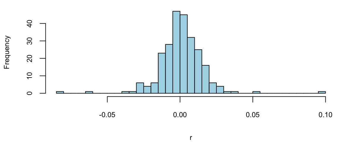
Example 9.3 (Google Stock Returns) Figure 9.2 shows the scattershot of Google and S&P 500 daily returns

Code

goog = read.csv("../../data/GOOG2019.csv") 
rgoog = goog$Adj.Close[2:251]/goog$Adj.Close[1:250] - 1 
sp = read.csv("../../data/SP2019.csv");   rsp = sp$Adj.Close[2:251]/sp$Adj.Close[1:250] - 1 
plot(rgoog, rsp, col="lightblue", pch=21, bg="grey", xlab="GOOG return", ylab="SP500 return") 

Figure 9.2: Scattershot of Google and S&P 500 daily returns

Let’s calculate the covariance and correlation between the daily returns of the Google stock and S&P 500.

Code

var_goog = mean((rgoog - mean(rgoog))^2) 
var_sp = mean((rsp - mean(rsp))^2) 
cov = mean((rgoog - mean(rgoog))*(rsp - mean(rsp))); print(cov) 

 8e-05

Code

cor = cov/(sqrt(var_goog)*sqrt(var_sp)); print(cor)

 0.67

Example 9.4 (Google Stock 2019) Consider observations of daily log-returns of a Google stock for 2019 Daily log-return on day \(t\) is calculated by taking a logarithm of the ratio of price at close of day \(t\) and at close of day \(t-1\) \[ y_t = \log\left(\dfrac{P_t}{P_{t-1}}\right) \] For example on January 3 of 2017, the open price is 778.81 and close price was 786.140, then the log-return is \(\log(786.140/778.81) = -0.0094\). It was empirically observed that log-returns follow a Normal distribution. This observation is a basis for Black-Scholes model with is used to evaluate future returns of a stock.

Code

p = read.csv("../../data/GOOG2019.csv")$Adj.Close; n = length(p) 
r = log(p[2:n]/p[1:(n-1)]) 
hist(r, breaks=30, col="lightblue", main="")

Observations on the far right correspond to the days when positive news was released and on the far left correspond to bad news. Typically, those are days when the quarterly earnings reports are released.

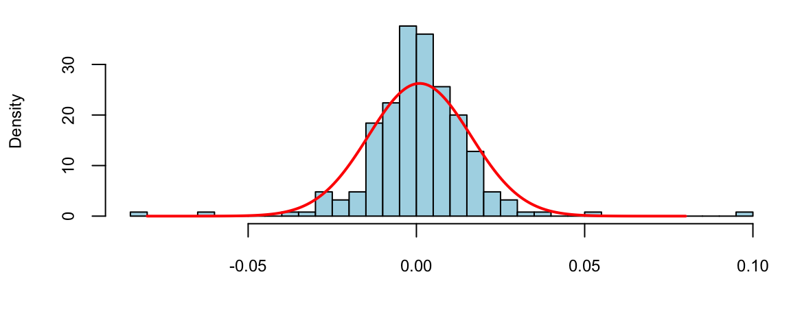
To estimate the expected value \(\mu\) (return) and standard deviation \(\sigma\) (a measure of risk), we simply calculate their sample counterparts \[ \bar{x} = \frac{1}{n} \sum_{i=1}^n x_i, ~\mathrm{ and }~ s^2 = \frac{1}{n-1} \sum_{i=1}^n (x_i - \bar{x} )^2 \] The empirical (or sample) values \(\bar x\) and \(s^2\) are called sample mean and sample variance. Here simply vie them as our best guess about the mean and variance of the normal distribution model then our probabilistic model for next day’s return is then given by \[ R \sim N(\bar x, s^2). \]

Say we are interested in investing into Google and would like to calculated the expected return of our investment as well as risk associated with this investment We assume that behavior of the returns in the future will be the same as in 2019.

n = length(r) 
rbar = sum(r)/n; print(rbar) 

 0.00098

s2 = sum((r-rbar)^2)/(n-1); print(s2) 

 0.00023

x = seq(-0.08,0.08, length.out = 200) 
hist(r, breaks=30, col="lightblue", freq = F, main="", xlab="") 
lines(x,dnorm(x,rbar,sqrt(s2)), col="red", lwd=2)

Histogram (blue) and fitted normal curve (red) of for the Google stock daily return data.

Now, assume, I invest all my portfolio into Google. I can predict my annual return to be \(251 \times 9.8\times 10^{-4}\) = 0.25 and risk (volatility) of my investment is \(\sqrt{s^2}\) = 0.02% a year.

I can predict the risk of loosing 3% or more in one day using my model is 1.93%.

pnorm(log(1-0.03), rbar, sqrt(s2))*100

 1.9

Code

sp = read.csv("../../data/SPMonthly.csv")$Adj.Close; n = length(sp) 
spret = sp[602:n]/sp[601:(n-1)]-1 # Calculate  1977-1987 returns 

mean(spret) 

 0.012

sd(spret)

 0.043

Altić, Mirela Slukan. 2013. “Exploring Along the Rome Meridian: Roger Boscovich and the First Modern Map of the Papal States.” In History of Cartography: International Symposium of the ICA, 2012, 71–89. Springer.

Bonfiglio, Rita, Annarita Granaglia, Raffaella Giocondo, Manuel Scimeca, and Elena Bonanno. 2021. “Molecular Aspects and Prognostic Significance of Microcalcifications in Human Pathology: A Narrative Review.” International Journal of Molecular Sciences 22 (120).

Feynman, Richard. n.d. “Feynman :: Rules of Chess.”

Halevy, Alon, Peter Norvig, and Fernando Pereira. 2009. “The Unreasonable Effectiveness of Data.” IEEE Intelligent Systems 24 (2): 8–12.

Nicosia, Luca, Giulia Gnocchi, Ilaria Gorini, Massimo Venturini, Federico Fontana, Filippo Pesapane, Ida Abiuso, et al. 2023. “History of Mammography: Analysis of Breast Imaging Diagnostic Achievements over the Last Century.” Healthcare 11 (1596).

Stigler, Stephen M. 1981. “Gauss and the Invention of Least Squares.” The Annals of Statistics, 465–74.