12 Logistic Regression
When the value \(y\) we are trying to predict is categorical (or qualitative) we have a classification problem. For a binary output we predict the probability its going to happen \[ p ( Y=1 | X = x ), \] where \(X = (x_1,\ldots,x_p)\) is our usual list of predictors.
Suppose that we have a binary response, \(y\) taking the value \(0\) or \(1\)
- Win or lose
- Sick or healthy
- Buy or not buy
- Pay or default
The goal is to predict the probability that \(y\) equals \(1\). You can then do and categorize a new data point. Assessing credit risk and default data is a typical problem. - \(y\): whether or not a customer defaults on their credit card (No or Yes). - \(x\): The average balance that customer has remaining on their credit card after making their monthly payment, plus as many other features you think might predict \(Y\).
A linear model is a powerful tool to find relations among different variables \[ y = \beta^Tx + \epsilon. \] It works assuming that \(y\) variable is contentious and ranges in \((-\infty,+\infty)\). Another assumption is that conditional distribution of \(y\) is normal \(p(y\mid \beta^Tx) \sim N(\beta^Tx, \sigma^2)\)
What do we do when assumptions about conditional normal distributions do not hold. For example \(y\) can be a binary variable with values 0 and 1. For example \(y\) is
- Outcome of an election
- Result of spam filter
- Decision variable about loan approval
We model response \(\{0,1\}\), using a continuous variable \(y \in [0,1]\) which is interpreted as the probability that response equals to 1. \[ p( y= 1 | x_1, \ldots , x_p ) = F \left ( \beta_1 x_1 + \ldots + b_p x_p \right ) \] where \(f\) is increasing and \(0< f(x)<1\).
It seems logical to find a transformation \(F\) so that \(F(\beta^Tx + \epsilon) \in [0,1]\). Then we can predict using \(F(\beta^Tx)\) and intercepting interpret the result as a probability, i.e if \(F(\beta^Tx) = z\) then we interpret it as \(p(y=1) = z\). Such function \(F\) is called a link function.
Do we know a function that maps any real number to a number in \([0,1]\) interval? What about commutative distribution function \(F(x) = p(Z \le x)\)? If we choose CDF \(\Phi(x)\) for \(N(0,1)\) then we have \[\begin{align*} \hat y = p(y=1) &= \Phi(\beta^Tx) \\ \Phi^{-1}(\hat y) = & \beta^Tx + \epsilon \end{align*}\] This is a linear model for \(\Phi^{-1}(\hat y)\), but not for \(y\)! You can thing of this as a change of units for variable \(y\). In this specific case, when we use normal CDF, the resulting model is called probit, it stands for probability unit. The resulting link function is \(\Phi^{-1}\) and now \(\Phi^{-1}(Y)\) follows a normal distribution! This term was coined in the 1930’s by biologists studying the dosage-cure rate link. We can fit a probit model using glm function in R.
Our prediction is the blue area which is equal to 0.0219.
A couple of observations: (i) this fits the data much better than the linear estimation, and (i) it always lies between 0 and 1. Instead of thinking of \(y\) as a probability and transforming right hand side of the linear model we can think of transforming \(y\) so that transformed variable lies in \((-\infty,+\infty)\). We can use odds ratio, that we talked about before \[ \dfrac{y}{1-y} \]
Odds ration lies in the interval \((0,+\infty)\). Almost what we need, but not exactly. Can we do another transform that maps \((0,+\infty)\) to \((-\infty,+\infty)\)? \[ \log\left(\dfrac{y}{1-y}\right) \] will do the trick! This function is called a logit function and it is This function is called a logit function and it is the inverse of the sigmoidal "logistic" function or logistic transform. The is linear in \[ \log \left ( \frac{ p \left ( y=1|x \right ) }{ 1 - p \left ( Y=1|x \right ) } \right ) = \beta_0 + \beta_1 x_1 + \ldots + x_p. \] These model are easy to fit in R:
glm( y ~ x1 + x2, family="binomial")
- is for indicates \(y=0\) or \(1\)
- has a bunch of other options.
Outside of specific field, i.e. behavioral economics, the logistic function is much more popular of a choice compared to probit model. Besides that fact that is more intuitive to work with logit transform, it also has several nice properties when we deal with multiple classes (more then 2). Also, it is computationally easier then working with normal distributions. The density function of the logit is very similar to the probit one.
We can easily derive an inverse of the logit function to get back the original \(y\) \[ \log\left(\dfrac{y}{1-y}\right) = \beta^Tx;~~ y=\dfrac{e^{\beta^Tx}}{1+e^{\beta^Tx}} \]
Example 12.1 (Example: NBA point spread)
Code
attach(NBA)
n = nrow(NBA)
hist(NBA$spread[favwin==1], col=5, main="", xlab="spread")
hist(NBA$spread[favwin==0], add=TRUE, col=6)
legend("topright", legend=c("favwin=1", "favwin=0"), fill=c(5,6), bty="n")
boxplot(NBA$spread ~ NBA$favwin, col=c(6,5), horizontal=TRUE, ylab="favwin", xlab="spread")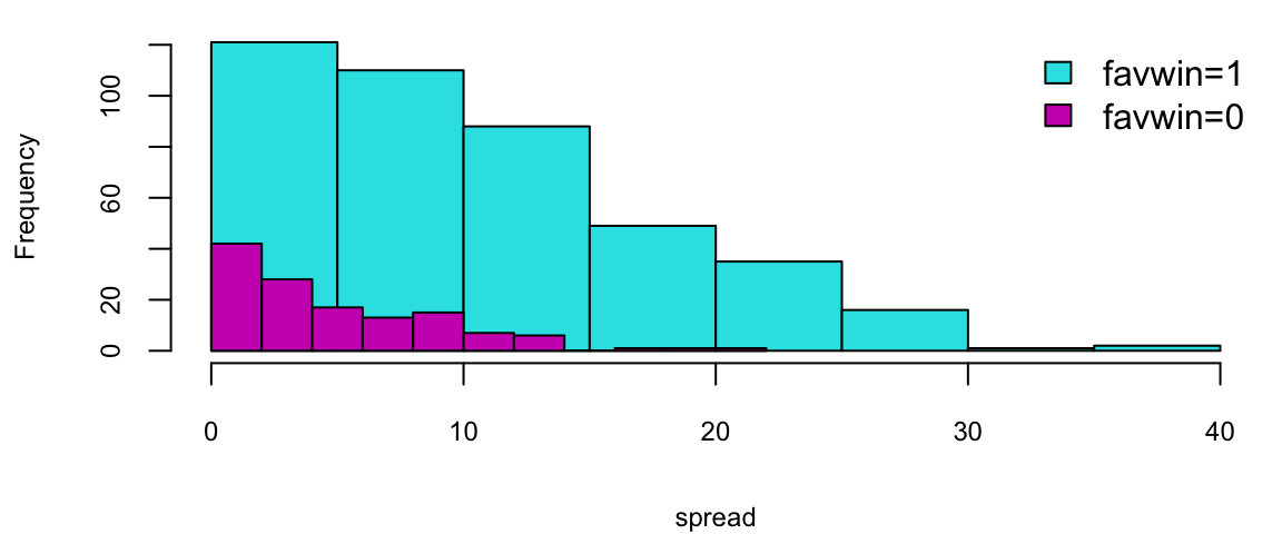
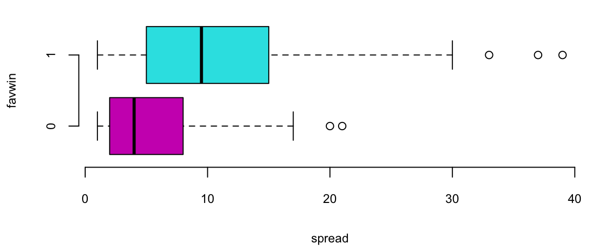
Does the Vegas point spread predict whether the favorite wins or not? Turquoise = Favorites does win, Purple = Favorite does not win. In R: the output gives us
Code
summary(nbareg)
Call:
glm(formula = favwin ~ spread - 1, family = binomial)

Coefficients:
       Estimate Std. Error z value Pr(>|z|)
spread   0.1560     0.0138    11.3   <2e-16 ***
---
Signif. codes:  0 '***' 0.001 '**' 0.01 '*' 0.05 '.' 0.1 ' ' 1

(Dispersion parameter for binomial family taken to be 1)

    Null deviance: 766.62  on 553  degrees of freedom
Residual deviance: 527.97  on 552  degrees of freedom
AIC: 530

Number of Fisher Scoring iterations: 5
Code
s = seq(0,30,length=100)
fit = exp(s*nbareg$coef[1])/(1+exp(s*nbareg$coef[1]))
plot(s, fit, typ="l", col=4, lwd=2, ylim=c(0.5,1), xlab="spread", ylab="P(favwin)")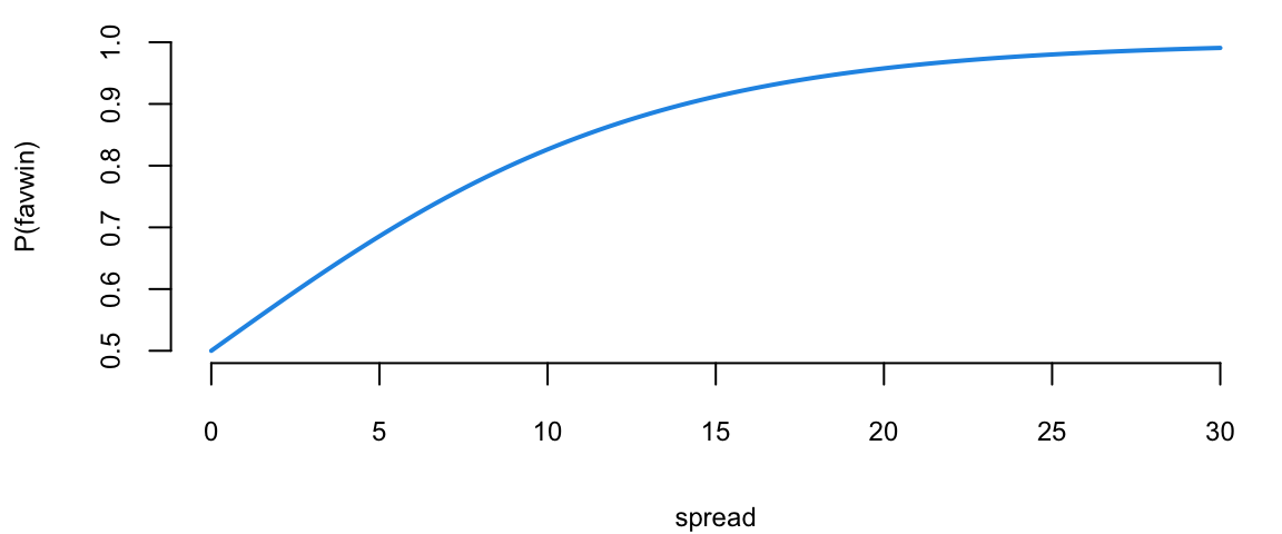
The \(\beta\) measures how our log-odds change! \(\beta = 0.156\)
Let’s do the NBA Point Spread Prediction. “Plug-in” the values for the new game into our logistic regression \[ { P \left ( \mathrm{ favwin} \mid \mathrm{ spread} \right ) = \frac{ e^{ \beta x } }{ 1 + e^{\beta x} } } \] Check that when \(\beta =0\) we have \(p= \frac{1}{2}\).
Given our new values spread\(=8\) or spread\(=4\), the win probabilities are \(77\)% and \(65\)%, respectively. Clearly, the bigger spread means a higher chance of winning.
Example 12.2 (Logistic Regression for Tennis Classification) Data science plays a major role in tennis, you can learn about recent AI tools developed by IBM from this This Yahoo Article.
We will analyze the Tennis Major Tournament Match Statistics Data Set from the UCI ML repository. The data set has one per each game from four major Tennis tournaments in 2013 (Australia Open, French Open, US Open, and Wimbledon).
Let’s load the data and familiarize ourselves with it
Code
dim(d) 943 44Code
str(d[,1:5])'data.frame': 943 obs. of 5 variables:
$ Player1: chr "Lukas Lacko" "Leonardo Mayer" "Marcos Baghdatis" "Dmitry Tu"..
$ Player2: chr "Novak Djokovic" "Albert Montanes" "Denis Istomin" "Michael "..
$ Round : int 1 1 1 1 1 1 1 1 1 1 ...
$ Result : int 0 1 0 1 0 0 0 1 0 1 ...
$ FNL1 : int 0 3 0 3 1 1 2 2 0 3 ...Let’s look at the few coluns of the randomly selected five rows of the data
Code
d[sample(1:943,size = 5),c("Player1","Player2","Round","Result","gender","surf")] Player1 Player2 Round Result gender surf
88 Andy Murray Vincent Millot 2 1 M Hard
773 T.Robredo N.Mahut 2 1 M Grass
836 K.Bertens Y.Shvedova 1 0 W Grass
418 Nadia Petrova Monica Puig 1 0 W Clay
549 Albert Montanes Edouard Roger-Vasselin 1 0 M HardWe have data for 943 matches and for each match we have 44 columns, including names of the players, their gender, surface type and match statistics. Let’s look at the number of break points won by each player. We will plot BPW (break points won) by each player on the scatter plot and will colorize each dot according to the outcome
Code
plot(d$BPW.1+rnorm(n),d$BPW.2+rnorm(n), pch=21, col=d$Result+2, cex=0.6, bg="yellow", lwd=0.8,
     xlab="BPW by Player 1", ylab="BPW by Player 2")
legend("bottomright", c("P1 won", "P2 won"), col=c(3,2), pch=21, bg="yellow", bty='n')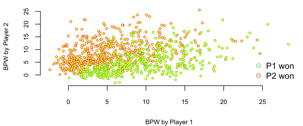
We can clearly see that number of the break points won is a clear predictor of the match outcome. Which is obvious and follows from the rules, to win a match, a player must win break points. Now, we want to understand the impact of a winning a break point on the overall match outcome. We do it by building a logistic regression model
Code
which(is.na(d$BPW.1)) # there is one row with NA value for the BPW.1 value and we remove it 171Code
d = d[-171,]; n = dim(d)[1]
m = glm(Result ~ BPW.1 + BPW.2-1, data=d, family = "binomial" )
summary(m)
Call:
glm(formula = Result ~ BPW.1 + BPW.2 - 1, family = "binomial",
    data = d)

Coefficients:
      Estimate Std. Error z value Pr(>|z|)
BPW.1   0.4019     0.0264    15.2   <2e-16 ***
BPW.2  -0.4183     0.0277   -15.1   <2e-16 ***
---
Signif. codes:  0 '***' 0.001 '**' 0.01 '*' 0.05 '.' 0.1 ' ' 1

(Dispersion parameter for binomial family taken to be 1)

    Null deviance: 1305.89  on 942  degrees of freedom
Residual deviance:  768.49  on 940  degrees of freedom
AIC: 772.5

Number of Fisher Scoring iterations: 5
R output does not tell us how accurate our model is but we can quickly check it by using the table function. We will use \(0.5\) as a threshold for our classification.
Code
table(d$Result, as.integer(m$fitted.values>0.5))
      0   1
  0 416  61
  1  65 400
Thus, our model got (416+416)/942 = 0.88% of the predictions correctly!
Essentially, the logistic regression is trying to draw a line that separates the red observations from the green one. In out case, we have two predictors \(x_1\) = BPW.1 and \(x_2\) = BPW.2 and our model is \[ \log\left(\dfrac{p}{1-p}\right) = \beta_1x_1 + \beta_2 x_2, \] where \(p\) is the probability of player 1 winning the match. We want to find the line along which the probability is 1/2, meaning that \(p/(1-p) = 1\) and log-odds \(\log(p/(1-p)) = 0\), thus the equation for the line is \(\beta_1x_1 + \beta_2 x_2 = 0\) or \[ x_2 = \dfrac{-\beta_1}{\beta_2}x_1 \]
Let’s see the line found by the glm function
Code
legend("bottomright", c("P1 won", "P2 won"), col=c(3,2), pch=21, bg="yellow", bty='n')

x = seq(0,30,length.out = 200)
y  =  -m$coefficients[1]*x/m$coefficients[2]
lines(x,y, lwd=2, col="red") 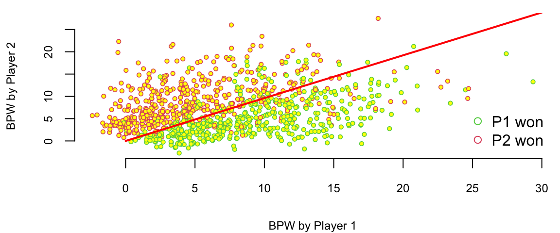
There are a couple of observations. First, effect of a break point on the game outcome is significant and symmetric, effect of loosing break point is the same as the effect of winning one. We also can interpret the effect of winning a break point in the following way. We will keep BPW.2 = 0 and will calculate what happens to the probability of winning when BPW.1 changes from 0 to 1. The odds ration for player 1 winning when BPW.1 = 0 is exp(0) which is 1, meaning that the probability that P1 wins is 1/2. Now when BPW.1 = 1, the odds ratio is 1.5
Code
exp(0.4019) 1.5We can calculate probability of winning from the regression equation \[
\dfrac{p}{1-p} = 1.5,~~~p = 1.5(1-p),~~~2.5p = 1.5,~~~p = 0.6
\] Thus probability of winning goes from 50% to 60%, we can use predict function to get this result
Code
predict.glm(m,newdata = data.frame(BPW.1 = c(0), BPW.2 = c(0)), type="response") 1
0.5 Code
predict.glm(m,newdata = data.frame(BPW.1 = c(1), BPW.2 = c(0)), type="response") 1
0.6 What happens to the chances of winning when P1 wins three more break points compared to the opponent
Code
predict.glm(m,newdata = data.frame(BPW.1 = c(0), BPW.2 = c(0)), type="response") 1
0.5 Code
predict.glm(m,newdata = data.frame(BPW.1 = c(3), BPW.2 = c(0)), type="response") 1
0.77 Chances go up by 27%.
Tennis is arguably the sport in which mean and women are treated equally. Both man and women matches are shown during the prime-time on TV, they both have the same prize money. However, one of the comments you hear often is that Women’s matches are “less predictable”, meaning that an upset (when the favorite looses) is more likely to happen in a women’s match compared to man Matches. We can test thus statement by looking at the residuals. The large the residual the less accurate our prediction was.
Code
outlind = which(d$res<2)
boxplot(d$res[outlind] ~ d$gender[outlind], col=c(2,3), xlab="Gender",ylab="Residual")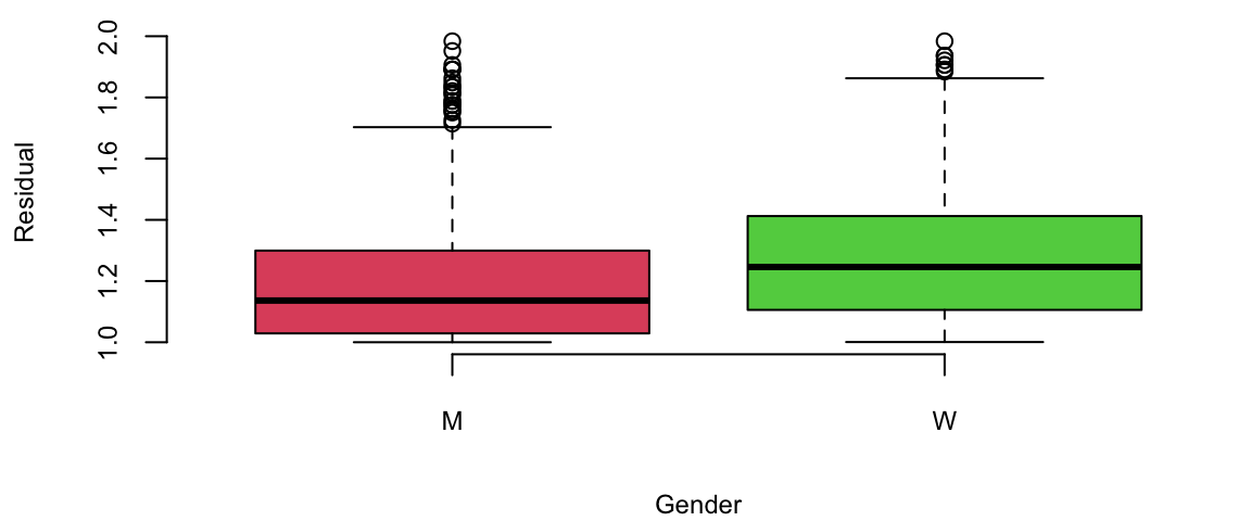
Let’s do a formal T-test on the residuals foe men’s and women’s matches
Code
men = d %>% filter(res<2, gender=="M") %>% pull(res)
women = d %>% filter(res<2, gender=="W") %>% pull(res)
t.test(men, women, alternative = "two.sided")
    Welch Two Sample t-test

data:  men and women
t = -5, df = 811, p-value = 3e-06
alternative hypothesis: true difference in means is not equal to 0
95 percent confidence interval:
 -0.105 -0.043
sample estimates:
mean of x mean of y
      1.2       1.3
Looks like the crowd wisdom that Women’s matches are less predictable is correct.
Example 12.3 (Credit Card Default) We have 10,000 observations
Code
Default = read.csv("../../data/CreditISLR.csv", stringsAsFactors = T)
head(Default)
default student balance income
1 No No 730 44362
2 No Yes 817 12106
3 No No 1074 31767
4 No No 529 35704
5 No No 786 38463
6 No Yes 920 7492Let’s build a logistic regression model
Code
glm.fit=glm(default~balance,data=Default,family=binomial)
summary(glm.fit)
Call:
glm(formula = default ~ balance, family = binomial, data = Default)

Coefficients:
             Estimate Std. Error z value Pr(>|z|)
(Intercept) -10.65133    0.36116   -29.5   <2e-16 ***
balance       0.00550    0.00022    24.9   <2e-16 ***
---
Signif. codes:  0 '***' 0.001 '**' 0.01 '*' 0.05 '.' 0.1 ' ' 1

(Dispersion parameter for binomial family taken to be 1)

    Null deviance: 2920.6  on 9999  degrees of freedom
Residual deviance: 1596.5  on 9998  degrees of freedom
AIC: 1600

Number of Fisher Scoring iterations: 8
We use it now to predict default
Code
predict.glm(glm.fit,newdata = list(balance=1000)) 1
-5.2 Code
-1.065e+01 + 5.499e-03*1000 -5.2Code
predict.glm(glm.fit,newdata = list(balance=1000), type="response") 1
0.0058 Code
exp(-1.065e+01 + 5.499e-03*1000)/(1+exp(-1.065e+01 + 5.499e-03*1000)) 0.0058Predicting default
Code
y = predict.glm(glm.fit,newdata = x, type="response")
plot(x$balance,y, pch=20, col="red", xlab = "balance", ylab="Default")
lines(Default$balance, as.integer(Default$default)-1, type='p',pch=20)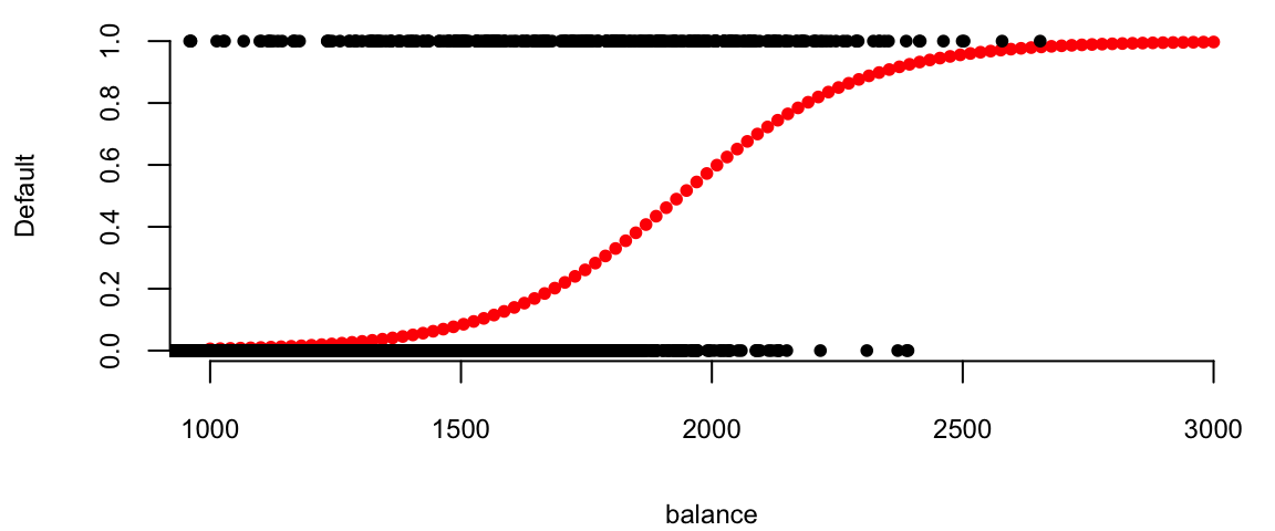
12.1 Confusion Matrix
We can use accuracy rate: \[ \text{accuracy} = \dfrac{\text{\# of Correct answers}}{n} \] or its dual, error rate \[ \text{error rate} = 1 - \text{accuracy}. \] You remember, we haw two types of errors. We can use confusion matrix to quantify those
| Predicted: YES | Predicted: NO | |
|---|---|---|
| Actual: YES | TPR | FNR |
| Actual: NO | FPR | TNR |
True positive rate (TPR) is the sensitivity and false positive rate (FPR) is the specificity of our predictive model
Example: Evolute the previous model Accuracy = 0.96
| Predicted: YES | Predicted: NO | |
|---|---|---|
| Actual: YES | TPR=0.6 | FNR=0.4 |
| Actual: NO | FPR=0.03 | TNR=0.97 |
I used \(p=0.2\) as a cut-off. What if I use smaller or larger \(p\), e.g. \(p=0\)?
ROC Curve Shows what happens for different cut-off values
First, we define a function, that calculates the ROC
Code
roc <- function(p,y, ...){
  y <- factor(y)
  n <- length(p)
  p <- as.vector(p)
  Q <- p > matrix(rep(seq(0,1,length=100),n),ncol=100,byrow=TRUE)
  specificity <- colMeans(!Q[y==levels(y)[1],])
  sensitivity <- colMeans(Q[y==levels(y)[2],])
  plot(1-specificity, sensitivity, type="l", ...)
  abline(a=0,b=1,lty=2,col=8)
}
Code
## roc curve and fitted distributions
pred = predict.glm(glm.fit,newdata = Default, type="response")
default = y
roc(p=pred, y=Default$default, bty="n", main="in-sample")
# our 1/5 rule cutoff
points(x= 1-mean((pred<.2)[default==0]),
       y=mean((pred>.2)[default==1]),
       cex=1.5, pch=20, col='red')
## a standard `max prob' (p=.5) rule
points(x= 1-mean((pred<.5)[default==0]),
       y=mean((pred>.5)[default==1]),
       cex=1.5, pch=20, col='blue')
legend("bottomright",fill=c("red","blue"),
       legend=c("p=1/5","p=1/2"),bty="n",title="cutoff")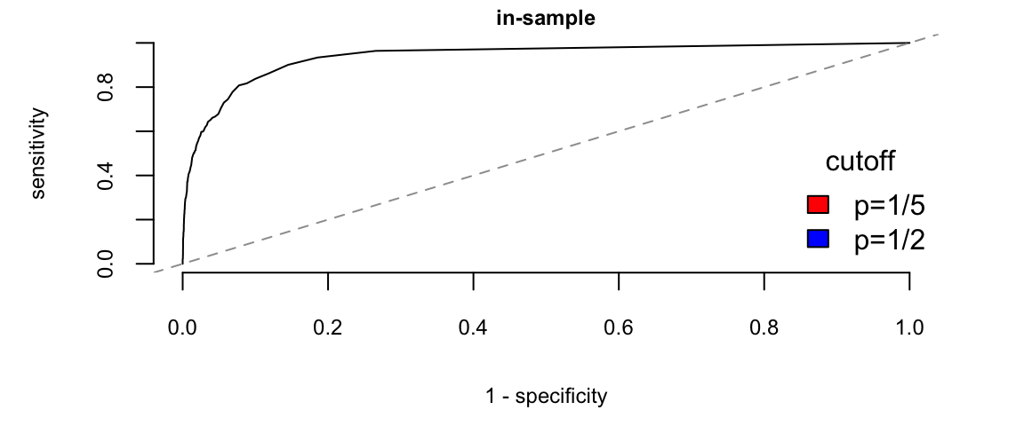
Look at other predictors
Code
glm.fit=glm(default~balance+income+student,data=Default,family=binomial)
summary(glm.fit)
Call:
glm(formula = default ~ balance + income + student, family = binomial,
    data = Default)

Coefficients:
             Estimate Std. Error z value Pr(>|z|)
(Intercept) -1.09e+01   4.92e-01  -22.08   <2e-16 ***
balance      5.74e-03   2.32e-04   24.74   <2e-16 ***
income       3.03e-06   8.20e-06    0.37   0.7115
studentYes  -6.47e-01   2.36e-01   -2.74   0.0062 **
---
Signif. codes:  0 '***' 0.001 '**' 0.01 '*' 0.05 '.' 0.1 ' ' 1

(Dispersion parameter for binomial family taken to be 1)

    Null deviance: 2920.6  on 9999  degrees of freedom
Residual deviance: 1571.5  on 9996  degrees of freedom
AIC: 1580

Number of Fisher Scoring iterations: 8
Student is significant!?
Student vs Balance
Code
boxplot(balance~student,data=Default, col = Default$student, ylab = "balance")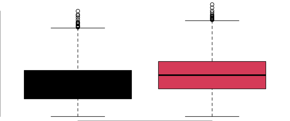
Let’s adjust for balance
Code
x2 = data.frame(balance = seq(1000,2500,length.out = 100), student = as.factor(rep("No",100)), income=rep(40,100))
y1 = predict.glm(glm.fit,newdata = x1, type="response")
y2 = predict.glm(glm.fit,newdata = x2, type="response")
plot(x1$balance,y1, type='l', col="red", xlab="Balance", ylab = "P(Default)")
lines(x2$balance,y2, type='l', col="black")
legend("topleft",bty="n", legend=c("Not Student", "Student"), col=c("black","red"), lwd=2)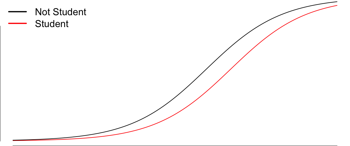
12.1.1 Estimating the Regression Coefficients
The coefficients \(\beta = (\beta_0, \beta_1)\) can be estimated using maximum likelihood method we discussed when talked about linear regression.
The model we derived above, gives us probability of \(y\), given \(x\) \[ p(y\mid x) = \dfrac{e^{\beta^Tx}}{1+e^{\beta^Tx}} \]
Now the problem is as follows \[ \underset{\beta}{maximize} \prod_{i:y_i = 1}p(x_i)\prod_{j:y_j = 0}(1-p(x_j)). \]
Maximum likelihood is a very general approach that is used to fit many of the non-linear models.
12.1.2 Choosing \(p\) and Evaluating Quality of Classifier
In logistic regression we use the logistic function to calculate a probability of \(y = 1\) \[ p(y=1\mid x) = \dfrac{e^{\beta^Tx}}{1+e^{\beta^Tx}}. \] Then, to predict a label we use a rule if \(y<p\), predict 0, and predict 1 otherwise. Now we answer the question of how to choose the cut-off value \(p\). We show it through an example.
Example 12.4 (Load Default) Assume a bank is using a logistic regression model to predict probability of a loan default and would issue a loan if \(a = p(y=1) < p\). Here \(p\) is the level of risk bank is willing to take. If bank chooses \(p=1\) and gives loans to everyone it is likely to loose a lot of money from defaulted accounts. If it chooses \(p = 0\) it will not issue loan to anyone and wont make any money. In order to choose an appropriate \(p\), we need to know what are the risks. Assume, bank makes $0.25 on every $1 borrowed in interest in fees and loose the entire amount of $1 if account defaults. This leads to the following pay-off matrix
| payer | defaulter | |
|---|---|---|
| loan | -0.25 | 1 |
| no load | 0 | 0 |
Then, given \(a = p(y=1)\), the expected profit is profit = \(0.25(1-a) - a\) to maintain a positive profit we need to choose \[ 0.25(1-a) - a >0 \iff -1.25a > -0.25 \iff a < 0.25 /1.25= 0.2 \] Thus, by choosing cutoff to be 0.2 or less, we guarantee to make profit on our loans.
To evaluate a binary classification predictor, we will use confusion matrix. It is shows numbers of correct predictions by the model (true positives and true negatives) and incorrect ones (false positive and false negatives). Say, we have a model that predicts weather person has a disease or not and we evaluate this model using 200 samples (\(n=200\)) with 60 being labeled as 0 (NO) and 140 labeled as 1 (YES) and model predicted correctly 130 YES labeled observations and 50 NOs.
| Predicted: YES | Predicted: NO | |
|---|---|---|
| Actual: YES | TP = 130 | FN = 10 |
| Actual: NO | FP = 10 | TN = 50 |
Sometimes, it is convenient to used rates rather than absolute counts and we compute
| Predicted: YES | Predicted: NO | |
|---|---|---|
| Actual: YES | TPR = 130/140 | FNR = 10/140 |
| Actual: NO | FPR = 10/60 | TNR = 50/60 |
True positive rate (TPR) is nothing but the sensitivity and false positive rate (FPR) is the specificity of our predictive model. Accuracy, which is the percent of correct predictions is another metric can be used to evaluate a classifier. \[ \mbox{Accuracy} = \dfrac{\mbox{TP + TN}}{n}. \] The error rate is opposite to accuracy \[ \mbox{Error rate} = 1- \mbox{Accuracy} \]
For a logistic regression, the confusion matrix will be different for different choices of the cut-off values \(p\). If we would like to understand the performance of the model for different values of \(p\) we can split an ROC curve, which plots pairs of TPR and FPR for different values of \(p\). Saw we take a sequence of 11 values \(p \in {0, 0.1, 0.2,\ldots,1}\) and we evaluate TPR and FPR for those 10 values and plot those pairs on a 2D plot then we will get the ROC curve. A few facts about the ROC curve:
- If we set \(p=0\), then any model will always predict NO, this leads to FPR=0 and TPR=0
- If we set \(p=1\) and model always predicts YES, then we get FPR = 1 and TPR = 1
- If we have an “ideal" model then for any \(0<p<1\) we will have FPR = 0 and TPR = 1.
- A naive model that uses coin flip to classify will have FPR = 1/2 and TPR = 1/2
- An ROC curve for an model will lie in-between the ideal curve and naive curve. If your model is worse then naive, it is not a good model. And your model cannot be better than an ideal model.
Example 12.5 (Default) Let’s consider an example. We want to predict default given attributes of the loan applicant. We have 1000 observations of 9 variables
Code
credit = read.csv("../../data/credit.csv")
credit$history = factor(credit$history, levels=c("A30","A31","A32","A33","A34"))
levels(credit$history) = c("good","good","poor","poor","terrible")
credit$foreign <- factor(credit$foreign, levels=c("A201","A202"), labels=c("foreign","german"))
credit$rent <- factor(credit$housing=="A151")
credit$purpose <- factor(credit$purpose, levels=c("A40","A41","A42","A43","A44","A45","A46","A47","A48","A49","A410"))
levels(credit$purpose) <- c("newcar","usedcar",rep("goods/repair",4),"edu",NA,"edu","biz","biz")

credit <- credit[,c("Default", "duration", "amount",
                    "installment", "age", "history",
                    "purpose", "foreign", "rent")]
knitr::kable(head(credit))| Default | duration | amount | installment | age | history | purpose | foreign | rent |
|---|---|---|---|---|---|---|---|---|
| 0 | 6 | 1169 | 4 | 67 | terrible | goods/repair | foreign | FALSE |
| 1 | 48 | 5951 | 2 | 22 | poor | goods/repair | foreign | FALSE |
| 0 | 12 | 2096 | 2 | 49 | terrible | edu | foreign | FALSE |
| 0 | 42 | 7882 | 2 | 45 | poor | goods/repair | foreign | FALSE |
| 1 | 24 | 4870 | 3 | 53 | poor | newcar | foreign | FALSE |
| 0 | 36 | 9055 | 2 | 35 | poor | edu | foreign | FALSE |
We build a logistic regression model using all of the 8 predictors and their interactions
credscore = glm(Default~.^2,data=credit,family=binomial)Then we plot ROC curve (FPR vs TPR) for different values of \(p\) and compare the curve with the naive
12.2 Multinomial logistic regression
Softmax regression (or multinomial logistic regression) is a generalization of logistic regression to the case where we want to handle multiple classes. In logistic regression we assumed that the labels were binary: \(y_i \in \{0,1\}\) . We used such a classifier to distinguish between two kinds of hand-written digits. Softmax regression allows us to handle \(y_i \in \{1,\ldots ,K\}\) where \(K\) is the number of classes. Our model took the form: \[ f(x\mid \beta)=\dfrac{1}{1+\exp(-\beta^Tx)}~, \] and the model parameters \(\beta\) were trained to minimize the loss function (negative log-likelihood) \[ J(\beta) = -\left[ \sum_{i=1}^m y_i \log f(x\mid \beta) + (1-y_i) \log (1-f(x\mid \beta)) \right] \]
Given a test input \(x\), we want our model to estimate the probability that \(p(y=k|x)\) for each value of \(k=1,\ldots ,K\) Thus, our model will output a \(K\)-dimensional vector (whose elements sum to 1) giving us our K estimated probabilities. Concretely, our model \(f(x\mid \beta)\) takes the form: \[ \begin{aligned} f(x\mid \beta) = \begin{bmatrix} p(y = 1 | x; \beta) \\ p(y = 2 | x; \beta) \\ \vdots \\ p(y = K | x; \beta) \end{bmatrix} = \frac{1}{ \sum_{j=1}^{K}{\exp(\beta_k^T x) }} \begin{bmatrix} \exp(\beta_1^{T} x ) \\ \exp(\beta_2^{T} x ) \\ \vdots \\ \exp(\beta_k^T x ) \\ \end{bmatrix}\end{aligned} \]
Here \(\beta_i \in R^n, i=1,\ldots,K\) are the parameters of our model. Notice that the term \(1/ \sum_{j=1}^{K}{\exp(\beta_k^T x) }\) normalizes the distribution, so that it sums to one.
For convenience, we will also write \(\beta\) to denote all the parameters of our model. When you implement softmax regression, it is usually convenient to represent \(\beta\) as an \(n\)-by-\(K\) matrix obtained by concatenating \(\beta_1,\beta_2,\ldots ,\beta_K\) into columns, so that \[ \beta = \left[\begin{array}{cccc}| & | & | & | \\ \beta_1 & \beta_2 & \cdots & \beta_K \\ | & | & | & | \end{array}\right]. \]
We now describe the cost function that we’ll use for softmax regression. In the equation below, \(1\) is the indicator function, so that \(1\)(a true statement)=1, and \(1\)(a false statement)=0. For example, 1(2+3 > 4) evaluates to 1; whereas 1(1+1 == 5) evaluates to 0. Our cost function will be: \[ \begin{aligned} J(\beta) = - \left[ \sum_{i=1}^{m} \sum_{k=1}^{K} 1\left\{y_i = k\right\} \log \frac{\exp(\beta_k^T x_i)}{\sum_{j=1}^K \exp(\beta_k^T x_i)}\right] \end{aligned} \]
Notice that this generalizes the logistic regression cost function, which could also have been written: \[ \begin{aligned} J(\beta) &= - \left[ \sum_{i=1}^m (1-y_i) \log (1-f(x\mid \beta)) + y_i \log f(x\mid \beta) \right] \\ &= - \left[ \sum_{i=1}^{m} \sum_{k=0}^{1} 1\left\{y_i = k\right\} \log p(y_i = k | x_i ; \beta) \right]\end{aligned} \] The softmax cost function is similar, except that we now sum over the \(K\) different possible values of the class label. Note also that in softmax regression, we have that \[ p(y_i = k | x_i ; \beta) = \frac{\exp(\beta_k^T x_i)}{\sum_{j=1}^K \exp(\beta_k^T x_i) }. \]
Softmax regression has an unusual property that it has a redundant set of parameters. To explain what this means, suppose we take each of our parameter vectors \(\beta_j\), and subtract some fixed vector \(\psi\). Our model now estimates the class label probabilities as \[ \begin{aligned} p(y_i = k | x_i ; \beta) &= \frac{\exp((\beta_k-\psi)^T x_i)}{\sum_{j=1}^K \exp( (\beta_j-\psi)^T x_i)} \\ &= \frac{\exp(\beta_k^T x_i) \exp(-\psi^T x_i)}{\sum_{j=1}^K \exp(\beta_k^T x_i) \exp(-\psi^T x_i)} \\ &= \frac{\exp(\beta_k^T x_i)}{\sum_{j=1}^K \exp(\beta_k^T x_i)}.\end{aligned} \] In other words, subtracting \(\psi\) does not affect our model’ predictions at all! This shows that softmax regression’s parameters are redundant. More formally, we say that our softmax model is overparameterized, meaning that for any model we might fit to the data, there are multiple parameter settings that give rise to exactly the same model function \(f(x \mid \beta)\) mapping from inputs \(x\) to the predictions.
Further, if the cost function \(J(\beta)\) is minimized by some setting of the parameters \((\beta_1,\ldots,\beta_K)\), then it is also minimized by \((\beta_1-\psi,\ldots,\beta_K-\psi)\) for any value of \(\psi\). Thus, the minimizer of \(J(\beta)\) is not unique. Interestingly, \(J(\beta)\) is still convex, and thus gradient descent will not run into local optima problems. But the Hessian is singular/non-invertible, which causes a straightforward implementation of Newton’s method to run into numerical problems. We can just set \(\psi\) to \(\beta_i\) and remove \(\beta_i\).
Example 12.6 (LinkedIn Study) How to Become an Executive(Irwin 2016; Gan and Fritzler 2016)?
Logistic regression was used to analyze the career paths of about \(459,000\) LinkedIn members who worked at a top 10 consultancy between 1990 and 2010 and became a VP, CXO, or partner at a company with at least 200 employees. About \(64,000\) members reached this milestone, \(\hat{p} = 0.1394\), conditional on making it into the database. The goals of the analysis were the following
- Look at their profiles – educational background, gender, work experience, and career transitions.
- Build a predictive model of the probability of becoming an executive
- Provide a tool for analysis of “what if” scenarios. For example, if you are to get a master’s degree, how your jobs perspectives change because of that.
Let’s build a logistic regression model with \(8\) key features (a.k.a. covariates): \[ \log\left ( \frac{p}{1-p} \right ) = \beta_0 + \beta_1x_1 + \beta_2x_2 + ... + \beta_8x_8 \]
\(p\): Probability of “success” – reach VP/CXO/Partner seniority at a company with at least 200 employees.
Features to predict the “success” probability: \(x_i (i=1,2,\ldots,8)\).
Variable Parameters \(x_1\) Metro region: whether a member has worked in one of the top 10 largest cities in the U.S. or globally. \(x_2\) Gender: Inferred from member names: ‘male’, or ‘female’ \(x_3\) Graduate education type: whether a member has an MBA from a top U.S. program / a non-top program / a top non-U.S. program / another advanced degree \(x_4\) Undergraduate education type: whether a member has attended a school from the U.S. News national university rankings / a top 10 liberal arts college /a top 10 non-U.S. school \(x_5\) Company count: # different companies in which a member has worked \(x_6\) Function count: # different job functions in which a member has worked \(x_7\) Industry sector count: # different industries in which a member has worked \(x_8\) Years of experience: # years of work experience, including years in consulting, for a member.
The following estimated \(\hat\beta\)s of features were obtained. With a sample size of 456,000 thy are measured rather accurately. Recall, given each location/education choice in the “Choice and Impact” is a unit change in the feature.
- Location: Metro region: 0.28
- Personal: Gender(Male): 0.31
- Education: Graduate education type: 1.16, Undergraduate education type: 0.22
- Work Experience: Company count: 0.14, Function count: 0.26, Industry sector count: -0.22, Years of experience: 0.09
Here are three main findings
- Working across job functions, like marketing or finance, is good. Each additional job function provides a boost that, on average, is equal to three years of work experience. Switching industries has a slight negative impact. Learning curve? lost relationships?
- MBAs are worth the investment. But pedigree matters. Top five program equivalent to \(13\) years of work experience!!!
- Location matters. For example, NYC helps.
We can also personalize the prediction for predict future possible future executives. For example, Person A (p=6%): Male in Tulsa, Oklahoma, Undergraduate degree, 1 job function for 3 companies in 3 industries, 15-year experience.
Person B (p=15%): Male in London, Undergraduate degree from top international school, Non-MBA Master, 2 different job functions for 2 companies in 2 industries, 15-year experience.
Person C (p=63%): Female in New York City, Top undergraduate program, Top MBA program, 4 different job functions for 4 companies in 1 industry, 15-year experience.
Let’s re-design Person B.
Person B (p=15%): Male in London, Undergraduate degree from top international school, Non-MBA Master, 2 different job functions for 2 companies in 2 industries, 15-year experience.
- Work in one industry rather than two. Increase \(3\)%
- Undergrad from top \(10\) US program rather than top international school. \(3\)%
- Worked for \(4\) companies rather than \(2\). Another \(4\)%
- Move from London to NYC. \(4\)%
- Four job functions rather than two. \(8\)%. A \(1.5\)x effect.
- Worked for \(10\) more years. \(15\)%. A \(2\)X effect.
Choices and Impact (Person B) are shown below 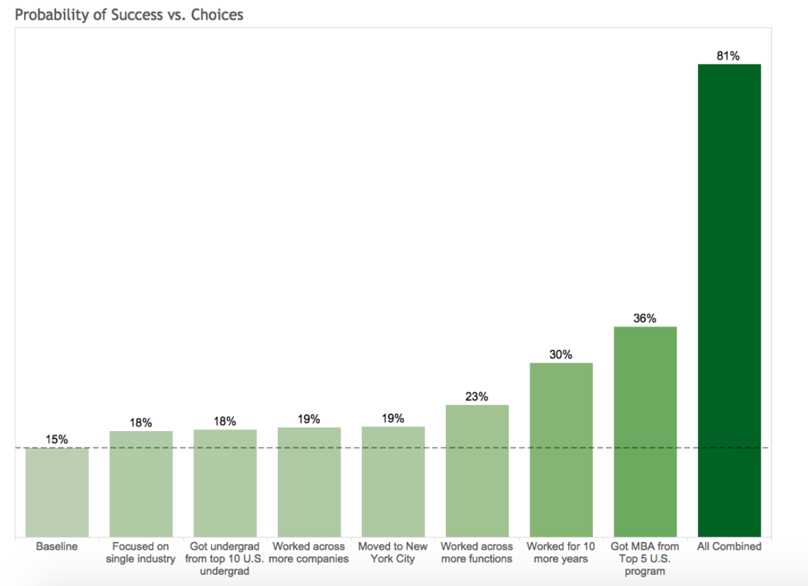
12.3 Imbalanced Data
Often, you have much more observations with a specific label, such a sample is called imbalanced. You should avoid using accuracy as a metric to choose a model. Say, you have a binary classification problem with 95% of samples labeled as 1. Then a naive classifier that assigns label 1 for each input will be 95% accurate. An ROC curve and area under the curve (AUC) metric derived from it should be used. Alternatively, you can use F1 sore, which combines precision and recall \[ F1 = 2\dfrac{\mathrm{precision} \times \mathrm{recall}}{\mathrm{precision} + \mathrm{recall}} \]
A modeler should consider synthetically generating more samples of class with small number of observation, e.g. bootstrap or using a generative model or subsampling observations with major label if data set is large enough.
12.4 Model Selection
A parametric model that we choose to fit to data is chosen from a family of functions. Then, we use optimization to find the best model from that family. To find the best model we either minimize empirical loss or maximize the likelihood. We also established, that when \(y \sim N(f(x\mid \beta),\sigma^2)\) then meas squared error loss and negative log-likelihood are the same function. \[ \E{y | x} = f(\beta^Tx) \]
For a regression model, an empirical loss measures a distance between fitted values and measurements and the goal is to minimize it. A typical choice of loss function for regression is \[ L (y,\hat y) = \dfrac{1}{n}\sum_{i=1}^n |y_i - f(\beta^Tx_i)|^p \] When \(p=1\) we have MAE (mean absolute error), \(p=2\) we have MSE (mean squared error).
Finding an appropriate family of functions is a major problem and is called model selection problem. For example, the choice of input variable to be included in the model is part of the model choice process. In practice we can find several models for the same data set that perform nearly identically. To summarize, the properties of a good model are
- Good model is not the one that fits data very well
- By including enough parameters we can make fit as close as we need
- Can have perfect fit when number of observations = number of parameters
- The goal not only to get a good fit but also to reduce complexity
- Model selection: do not include parameters we do not need
- Usually select a model from a relevant class
When we select a model for our analysis, we need to keep the following goals in mind - When we have many predictors (with many possible interactions), it can be difficult to find a good model. - Which input variables do we include? - Which interactions do we include? - Model selection tries to “simplify” this task.
The model selection task is sometimes one of the most consuming parts of the data analysis. Unfortunately, there is no single rule to find the best model. One way to think about the model choice problem as yet another optimization problem, with the goal to find best family of functions that describe the data. With a small number of predictors we can do brute force (check all possible models). For example, with \(p\) predictors there are \(2^p\) possible models with no interactions. Thus, the number of potential family functions is huge even for modest values of \(p\). One cannot consider all transformations and interactions.
12.4.1 Out of Sample Performance
Our goal is to build a model that predicts well for out-of-sample data, e.g. the data that was not used for training. Eventually, we are interested in using our models for prediction and thus, the out of sample performance is the most important metric and should be used to choose the final model. In-sample performance is of little interest when predictive model need to be chosen, as one of the winners of Netflix prize put it, “It’s like predicting how much someone will like a movie, having them watch it and tell you how much they really liked it”. The out-of-sample performance is the final judge of the quality of our model. The goal is to use data to find a pattern that we can exploit. The pattern will be “statistical" in its nature. To uncover the pattern we start with a training dataset, denoted by \[ D = (y_i,x_i)_{i=1}^n \] and to test the validity of our mode we use out-of-sample testing dataset \[ D^* = (y_j^*, x_j^*)_{j=1}^m, \] where \(x_i\) is a set of \(p\) predictors ans \(y_i\) is response variable.
A good predictor will “generalize” well and provide low MSE out-of-sample. These are a number of methods/objective functions that we will use to find, \(\hat f\). In a parameter-based style we will find a black box. There are a number of ways to build our black box model. Our goal is to find the map \(f\) that approximates the process that generated the data. For example data could be representing some physical observations and our goal is recover the “laws of nature" that led to those observations. One of the pitfalls is to find a map \(f\) that does not generalize. Generalization means that our model actually did learn the”laws of nature" and not just identified patterns presented in training. The lack of generalization of the model is called over-fitting. It can be demonstrated in one dimension by remembering the fact from calculus that any set of \(n\) points can be approximated by a polynomial of degree \(n\), e.g we can alway draw a line that connects two points. Thus, in one dimension we can always find a function with zero empirical risk. However, such a function is unlikely to generalize to the observations that were not in our training data. In other words, the empirical risk measure for \(D^*\) is likely to be very high. Let us illustrate that in-sample fit can be deceiving.
Example 12.7 (Hard Function) Example: Say we want to approximate the following function \[ f(x) = \dfrac{1}{1+25x^2}. \] This function is simply a ratio of two polynomial functions and we will try to build a liner model to reconstruct this function
Figure 12.1 shows the function itself (black line) on the interval \([-3,3]\). We used observations of \(x\) from the interval \([-2,2]\) to train the data (solid line) and from \([-3,-2) \cup (2,3]\) (dotted line) to test the model and measure the out-of-sample performance. We tried four different linear functions to capture the relations. We see that linear model \(\hat y = \beta_0 + \beta_1 x\) is not a good model. However, as we increas the degree of the polynomial to 20, the resulting model \(\hat y = \beta_0 + \beta_1x + \beta_2 x^2 +\ldots+\beta_{20}x^{20}\) does fit the training data set quite well, but does very poor job on the test data set. Thus, while in-sample performance is good, the out-of sample performance is unsatisfactory. We should not use the degree 20 polynomial function as a predictive model. In practice in-sample out-of-simple loss or classification rates provide us with a metric for providing horse race between different predictors. It is worth mentioning here there should be a penalty for overly complex rules which fits extremely well in sample but perform poorly on out-of-sample data. As Einstein famous said “model should be simple, but not simpler.”
12.5 Bias-Variance Trade-off
Example 12.8 (Stein’s Paradox) Stein’s paradox, as explained Efron and Morris (1977), is a phenomenon in statistics that challenges our intuitive understanding of estimation. The paradox arises when trying to estimate the mean of a multivariate normal distribution. Traditionally, the best guess about the future is usually obtained by computing the average of past events. However, Charles Stein showed that there are circumstances where there are estimators better than the arithmetic average. This is what’s known as Stein’s paradox.
In 1961, James and Stein exhibited an estimator of the mean of a multivariate normal distribution that has uniformly lower mean squared error than the sample mean. This estimator is reviewed briefly in an empirical Bayes context. Stein’s rule and its generalizations are then applied to predict baseball averages, to estimate toxomosis prevalence rates, and to estimate the exact size of Pearson’s chi-square test with results from a computer simulation.
In each of these examples, the mean square error of these rules is less than half that of the sample mean. This result is paradoxical because it contradicts the elementary law of statistical theory. The philosophical implications of Stein’s paradox are also significant. It has influenced the development of shrinkage estimators and has connections to Bayesianism and model selection criteria.
We reproduce the baseball bartting average example from Efron and Morris (1977). The data is available in the R package Lahman. We will use the data from 2016 season.
Code
library(Lahman)Suppose that we have \(n\) independent observations \(y_{1},\ldots,y_{n}\) from a \(N\left( \theta,\sigma^{2}\right)\) distribution. The maximum likelihood estimator is \(\widehat{\theta}=\bar{y}\), the sample mean. The Bayes estimator is the posterior mean, \(\widehat{\theta}=\mathbb{E}\left[ \theta\mid y\right] =\frac{\sigma^{2}}{\sigma^{2}+n}% \bar{y}\). The Bayes estimator is a shrinkage estimator, it shrinks the MLE towards the prior mean. The amount of shrinkage is determined by the ratio of the variance of the prior and the variance of the likelihood. The Bayes estimator is also a function of the MLE, \(\widehat{\theta}=\frac{\sigma^{2}}{\sigma^{2}+n}\bar{y}+\frac{n}{\sigma^{2}+n}\widehat{\theta}\). This is a general property of Bayes estimators, they are functions of the MLE. This is a consequence of the fact that the posterior distribution is a function of the likelihood and the prior. The Bayes estimator is a function of the MLE, \(\widehat{\theta}=\frac{\sigma^{2}}{\sigma^{2}+n}\bar{y}+\frac{n}{\sigma^{2}+n}\widehat{\theta}\). This is a general property of Bayes estimators, they are functions of the MLE. This is a consequence of the fact that the posterior distribution is a function of the likelihood and the prior.
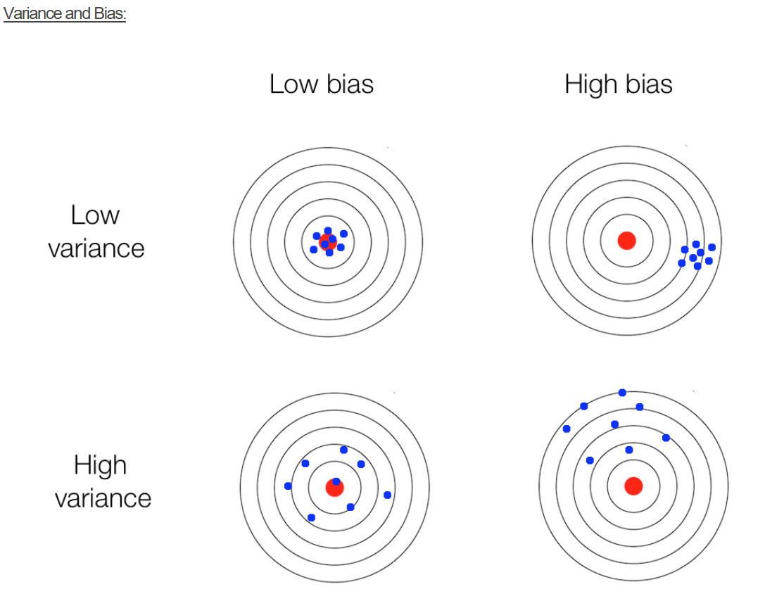
For any predictive model we seek to achieve best possible results, i.e. smallest MSE or misclassification rate. However, a model performance can be different as data used in one training/validation split may produce results dissimilar to another random split. In addition, a model that performed well on the test set may not produce good results given additional data. Sometimes we observe a situation, when a small change in the data leads to large change in the final estimated model, e.g. parameters of the model. These results exemplify the bias/variance tradeoff, where increasing model bias produces large variance in the final results. Similarly, low bias results in low variance, but can also produce an oversimplification of the final model. While Bias/variance concept is depicted below.
Example 12.9 (Bias-variance) We demonstrate bias-variance concept using Boston housing example. We fit a model \(\mathrm{medv} = f(\mathrm{lstat})\). We use polynomial functions to approximate this relation. We fitted twelve polynomial functions with degree \(1,\ldots,12\) ten time. Each time we randomly selected 20% of sample for testing and the rest for training. We estimated in-of-sample performance (bias) and out-of-sample performance by calculating MSE on training and testing sets correspondingly. For each polynomial \(f\) we averaged MSE from each of the ten models.
Figure 12.2 shows bias and variance for our twelve different models. As expected, bias increases while variance increases as model complexity grows. On the other hand out-of-sample MSE is a U-shaped curve. The optimal model is the one that has smallest out-of-sample MSE. In our case it is polynomial of degree 5!
Let’s take another, a more formal, look at bias-variance trade-off for a linear regression problem. We are interested in the decomposition of the error \(\E{(y-\hat y)^2}\) as a function of bias \(\E{y-\hat y}\) and variance \(\Var{\hat y}\).
Here \(\hat y = \hat f_{\beta}(x)\) prediction from the model, and \(y = f(x) + \epsilon\) is the true value, which is measured with noise \(\Var{\epsilon} = \sigma^2\), \(f(x)\) is the true unknown function. The expectation above measures squared error of our model on a random sample \(x\). \[ \begin{aligned} \E{(y - \hat{y})^2} & = \E{y^2 + \hat{y}^2 - 2 y\hat{y}} \\ & = \E{y^2} + \E{\hat{y}^2} - \E{2y\hat{y}} \\ & = \Var{y} + \E{y}^2 + \Var{\hat{y}} + \E{\hat{y}}^2 - 2f\E{\hat{y}} \\ & = \Var{y} + \Var{\hat{y}} + (f^2 - 2f\E{\hat{y}} + \E{\hat{y}}^2) \\ & = \Var{y} + \Var{\hat{y}} + (f - \E{\hat{y}})^2 \\ & = \sigma^2 + \Var{\hat{y}} + \mathrm{Bias}(\hat{y})^2\end{aligned} \] Here we used the following identity: \(\Var{X} = \E{X^2} - \E{X}^2\) and the fact that \(f\) is deterministic and \(\E{\epsilon} = 0\), thus \(\E{y} = \E{f(x)+\epsilon} = f + \E{\epsilon} = f\).
12.6 Cross-Validation
If the data set at-hand is small and we cannot dedicate large enough sample size for testing, simply measuring error on test data set can lead to wrong conclusions. When size of the testing set \(D^*\) is small, the estimated out-of-sample performance is of high variance, depending on precisely which observations are included in the test set. On the other hand, when training set \(D^*\) is a large fraction of the entire sample available, estimated out-of-sample performance will be underestimated. Why?
A trivial solution is to perform the training/testing split randomly several times and then use average out-of-sample errors. This procedure has two parameters, the fraction of samples to be selected for testing \(p\) and number of estimates to be performed \(K\). The resulting algorithm is as follows
fsz = as.integer(p*n)
error = rep(0,K)
for (k in 1:K)
{
    test_ind = sample(1:n,size = fsz)
    training = d[-test_ind,]
    testing  = d[test_ind,]
    m = lm(y~x, data=training)
    yhat = predict(m,newdata = testing)
    error[k] = mean((yhat-testing$y)^2)
}
res = mean(error)Figure[fig:cv](a) shows the process of splitting data set randomly five times.
Cross validation modifies the random splitting approach uses more “disciplined” way to split data set for training and testing. Instead of randomly selecting training data points, CV chooses consecutive observations and thus, each data point is used once for testing. As the random approach, CV helps addressing the high variance issue of out-of-sample performance estimation when data set available is small. Figure[fig:cv](b) shows the process of splitting data set five times using cross-validation approach.
Training set (red) and testing set (green) from (a) cross-validation and (b) bootstrap.
Example 12.10 (Simulated) We use simulated data set to demonstrate difference between estimated out-of-sample performance using random 20/80 split, 5-fold cross-validation and random split. We used \(x=-2,-1.99,-1.98,\ldots,2\) and \(y = 2+3x + \epsilon, ~ \epsilon \sim N(0,\sqrt{3})\). We simulated 35 datasets of size 100. For each of the simulated data sets, we fitted a linear model and estimated out-of-sample performance using three different approaches. Figure[fig:test-error20] compares empirical distribution of errors estimated from 35 samples.
As we can see the estimated out-of-sample performance by a training set approach is of high variance. While, both cross-validation and bootstrap approaches lead to better estimates, they require model to be fitted 5 times, which can be computationally costly for a complex model. On the other hand, estimate from cross-validation is of lower variance and less bias compared to the bootstrap estimate. Thus, we should prefer cross-validation.
12.7 Small Sample Size
When sample size is small and it is not feasible to divide your data into training and validation data sets, an information criterion could be used to assess a model. We can think of information criterion as a metric that “approximates” out-os-sample performance of the model. Akaike’s Information Criterion (AIC) takes the form \[ \mathrm{AIC} = log(\sigma_k^2) + \dfrac{n+2k}{n} \] \[ \hat{\sigma}_k^2 = \dfrac{SSE_k}{n} \] Here \(k\) = number of coefficients in regression model, \(SSE_k\) = residual sum of square, \(\hat{\sigma}_k^2\) = MLE estimator for variance. We do not need to proceed sequentially, each model individually evaluated
AIC is derived using the Kullback-Leibler information number. It is a ruler to measure the similarity between the statistical model and the true distribution. \[ I(g ; f) = E_g\left(\log \left\{\dfrac{g(y)}{f(y)}\right\}\right) = \int_{-\infty}^{\infty}\log \left\{\dfrac{g(y)}{f(y)}\right\}g(y)dy. \] Here - \(I(g ; f) > 0\) - \(I(g ; f) = 0 \iff g(u) = f(y)\) - \(f \rightarrow g\) as \(I(g ; f) \rightarrow 0\)
To estimate \(I(g ; f)\), we write \[ I(g ; f) = E_g\left(\log \left\{\dfrac{g(y)}{f(y)}\right\}\right) = E_g (\log g(y)) - E_g(\log f(y)) \] Only the second term is important in evaluating the statistical model \(f(y)\). Thus we need to estimate \(E_g(\log f(y))\). Given sample \(z_1,...,z_n\), and estimated parameters \(\hat{\theta}\) a naive estimate is \[ \hat{E}_g(\log f(y)) = \dfrac{1}{n} \sum_{i=1}^n \log f(z_i) = \dfrac{\ell(\hat{\theta})}{n} \] where \(\ell(\hat{\theta})\) is the log-likelihood function for model under test.
- this estimate is very biased
- data used used twice: to get the MLE and second to estimate the integral
- it will favor those model that overfit
Akaike showed that the bias is approximately \(k/n\) where \(k\) is the number of parameters \(\theta\). Therefore we use \[ \hat{E}_g(\log f(y)) = \dfrac{\ell(\hat{\theta})}{n} - \dfrac{k}{n} \] Which leads to AIC \[ AIC = 2n \hat{E}_g(\log f(y)) = 2 \ell(\hat{\theta}) - 2k \]
Akaike’s Information Criterion (AIC) \[ \mathrm{AIC} = \log(\sigma_k^2) + \dfrac{n+2k}{n} \] Controls for alance between model complexity (\(k\)) and minimizing variance. The model selection process involve trying different \(k\), chose model with smallest AIC.
A slightly modified version designed for small samples is the bias corrected AIC (AICc). \[ \mathrm{AICc} = \log(\hat{\sigma}_k^2) + \dfrac{n+k}{n-k-2} \] This criterion should be used for regression models with small samples
Yet, another variation designed for larger datasets is the Bayesian Information Criterion (BIC). \[ \mathrm{BIC} = \log(\hat{\sigma}_k^2) + \dfrac{k \log(n)}{n} \] Is is the same as AIC but harsher penalty, this chooses simpler models. It works better for large samples when compared to AICc. The motivation fo BIC is from the posterior distribution over model space. Bayes rule lets you calculate the joint probability of parameter and models as \[ p(\theta,M\mid D) = \dfrac{p(D\mid \theta,M(p(M,\theta)}{p(D)},~~ p(M\mid D) = \int p(\theta,M\mid D)d\theta \approx n^{p/2}p(D\mid \hat \theta M)p(M). \]
Consider a problem of predicting mortality rates given pollution and temperature measurements. Let’s plot the data.
Comparison of (a) ideal scenario of an experiment being repeated many times and (b) bootstrap scenario when we simulate repeated experiments by re-sampling from existing sample
Regression Model 1, which just uses the trend: \(M_t = \beta_1 + \beta_2 t + w_t\). We fit by calling lm(formula = cmort ~ trend) to get the following coefficients
                Estimate    Std. Error t value
    (Intercept) 3297.6062   276.3132   11.93
    trend         -1.6249     0.1399  -11.61
Regression Model 2 regresses to time (trend) and temperature: \(M_t = \beta_1 + \beta_2 t + \beta_t(T_t - T)+ w_t\). The R call is lm(formula = cmort ~ trend + temp)
                Estimate    Std. Error t value
    (Intercept) 3125.75988  245.48233   12.73
    trend         -1.53785    0.12430  -12.37
    temp          -0.45792    0.03893  -11.76
Regression Model 3, uses trend, temperature and mortality: \(M_t = \beta_1 + \beta_2 t + \beta_3(T_t - T)+ \beta_4(T_t - T)^2 + w_t\). The R call is lm(formula = cmort ~ trend + temp + I(temp^2)
                Estimate    Std. Error t value
    (Intercept)  3.038e+03  2.322e+02  13.083
    trend       -1.494e+00  1.176e-01 -12.710
    temp        -4.808e-01  3.689e-02 -13.031
    temp2        2.583e-02  3.287e-03   7.858
Regression Model 4 adds temperature squared: \(M_t = \beta_1 + \beta_2 t + \beta_3(T_t - T)+ \beta_4(T_t - T)^2 + \beta_5 P_t+ w_t\). The R call is lm(formula = cmort ~ trend + temp + I(temp^2) + part)
                Estimate    Std. Error t value
    (Intercept)  2.831e+03  1.996e+02   14.19
    trend       -1.396e+00  1.010e-01  -13.82
    temp        -4.725e-01  3.162e-02  -14.94
    temp2        2.259e-02  2.827e-03    7.99
    part         2.554e-01  1.886e-02   13.54
To choose the model, we look at the information criterion
| Model | \(k\) | SSE | df | MSE | \(R^2\) | AIC | BIC |
|---|---|---|---|---|---|---|---|
| 1 | 2 | 40,020 | 506 | 79.0 | .21 | 5.38 | 5.40 |
| 2 | 3 | 31,413 | 505 | 62.2 | .38 | 5.14 | 5.17 |
| 3 | 4 | 27,985 | 504 | 55.5 | .45 | 5.03 | 5.07 |
| 4 | 5 | 20,508 | 503 | 40.8 | .60 | 4.72 | 4.77 |
\(R^2\) always decreases with number of covariates (that is what MLE does). Thus, cannot be used as a selection criteria. \(R^2\) for out-of-sample data is useful!
The message to take home on model selection
- \(R^2\) is NOT a good metric for model selection
- Value of likelihood function is NOT a god metric
- are intuitive and work very well in practice (you should use those)
- AIC is good for big \(n/df\), so it overfits in high dimensions
- Should prefer AICc over AIC
- BIC underfits for large \(n\)
- Cross-validation is important, we will go over it later
13 Regularization
Regularization is a technique to incorporate some prior knowledge about parameters of the model into the estimation process. Consider an example when regularization allows us to solve a hard problem of filtering noisy traffic data.
Example 13.1 (Traffic) Consider traffic flow speed measured by an in-ground sensor installed on interstate I-55 near Chicago. Speed measurements are noisy and prone to have outliers. Figure[fig:speed-profile] shows speed measured data, averaged over five minute intervals on one of the weekdays.
Speed measurements are noisy and prone to have outliers. There are two sources of noise. The first is the measurement noise, caused by inhalant nature of the sensor’s hardware. The second source is due to sampling error, vehicles observed on a specific lane where senor installed might not represent well traffic in other lanes.
Trend filtering, which is a variation of a well-know Hodrick-Prescott filter. In this case, the trend estimate is the minimizer of the weighted sum objective function \[(1/2) \sum_{t=1}^{n}(y_t - x_t)^2 + \lambda \sum_{t=1}^{n-1}|x_{t-1} - 2x_t + x_{t+1}|, \]
13.1 Ridge Regression
Gauss invented the concept of least squares and developed algorithms to solve the the optimization problem \[ \underset{\beta}{\mathrm{minimize}}\quad ||y- X\beta||_2^2 \] where \(\beta = (\beta_1 , \ldots , \beta_p )\), we can use linear algebra algorithms, the solution given by \[ \hat{\beta} = ( X^T X )^{-1} X^T y \] This can be numerically unstable when \(X^T X\) is ill-conditioned, and happens when \(p\) is large. Ridge regression addresses this problem by adding an extra term to the \(X^TX\) matrix \[ \hat{\beta}_{\text{ridge}} = ( X^T X + \lambda I )^{-1} X^T y. \] The corresponding optimization problem is \[ \underset{\beta}{\mathrm{minimize}}\quad ||y- X\beta||_2^2 + \lambda||\beta||_2^2. \] An alternative formulation is We can think of the constrain is of a budget on the size of \(\beta\).
The we choose \(\lambda\) over a regularisation path. The penalty in ridge regression forces coefficients \(\beta\) to be close to 0. Penalty is large for large values and very small for small ones. Tuning parameter \(\lambda\) controls trade-off between how well model fits the data and how small \(\beta\)s are. Different values of \(\lambda\) will lead to different models. We select \(\lambda\) using cross validation.
Example 13.2 (Shrinkage) Consider a simulated data with \(n=50\), \(p=30\), and \(\sigma^2=1\). The true model is linear with \(10\) large coefficients between \(0.5\) and \(1\).
Our approximators \(\hat f_{\beta}\) is a linear regression. We can empirically calculate the bias by calculating the empirical squared loss \(1/n||y -\hat y||_2^2\) and variance can be empirically calculated as \(1/n\sum (\bar{\hat{y}} - \hat y_i)\)
Bias squared \(\mathrm{Bias}(\hat{y})^2=0.006\) and variance \(\Var{\hat{y}} =0.627\). Thus, the prediction error = \(1 + 0.006 + 0.627 = 1.633\)
We’ll do better by shrinking the coefficients to reduce the variance. Let’s estimate, how big a gain will we get with Ridge?
Now we see the accuracy of the model as a function of \(\lambda\)
Ridge Regression At best: Bias squared \(=0.077\) and variance \(=0.402\).
Prediction error = \(1 + 0.077 + 0.403 = 1.48\)
The additional term \(\lambda||\beta||_2^2\) in the optimization problem is called the regularization term. There are several ways to regularize an optimization problem. All of those techniques were developed in the middle of last century and were applied to solve problems of fitting physics models into observed data, those frequently arise in physics and engineering applications. Here are a few examples of such regularization techniques.
Ivanov regularization \[ \underset{x \in \mathbb{R^n}}{\mathrm{minimize}}\quad ||y - X\beta||_2^2~~~~ \mbox{s.t.}~~||\beta||_l \le k \]
Morozov regularization \[ \underset{x \in \mathbb{R^n}{\mathrm{minimize}}\quad} ||\beta||_l~~~~ \mbox{s.t.}~~ ||y - X\beta||_2^2 \le \tau \] Here \(\tau\) reflects the so called noise level, i.e. an estimate of the error which is made during the measurement of \(b\).
Tikhonov regularization \[ \underset{\beta\in \mathbb{R^n}}{\mathrm{minimize}}\quad ||y - X\beta||_2^2 + \lambda||\beta||_l \] - Tikhonov regularization with \(l=1\) is lasso - Tikhonov regularization with \(l=2\) is ridge regression - lasso + ridge = elastic net
13.2 \(\ell_1\) Regularization (LASSO)
The Least Absolute Shrinkage and Selection Operator (LASSO) uses \(\ell_1\) norm penalty and in case of linear regression leads to the following optimization problem \[ \underset{\beta}{\mathrm{minimize}}\quad ||y- X\beta||_2^2 + \lambda||\beta||_1 \]
In one dimensional case solves the following optimization problem \[ \underset{\beta}{\mathrm{minimize}}\quad \frac{1}{2} (y-\beta)^2 + \lambda | \beta | \] The solution is given by the soft-thresholding operator defined by \[ \hat{\beta} = \mathrm{soft} (y; \lambda) = ( y - \lambda ~\mathrm{sgn}(y) )_+. \] Here sgn is the sign function and \(( x )_+ = \max (x,0)\). To demonstrate how this solution is derived, we can define a slack variable \(z = | \beta |\) and solve the joint constrained optimisation problem which is differentiable.
Graphically, the soft-thresholding operator is
LASSO has a nice feature that it forces some of the \(\hat{\beta}\)’s to zero. It is an automatic variable selection! Finding optimal solution is computationally fast, it is a convex optimisation problem, though, it is non-smooth. As in ridge regression, we still have to pick \(\lambda\) via cross-validation. Visually the process can be represented using regularization path graph, as in the following example Example: We model prostate cancer using LASSO
MSE and Regularization path for Prostate Cancer data
Now with ridge regression
MSE and Regularization path for Prostate Cancer data
Example 13.3 (Horse race prediction using logistic regression) We use the run.csv data from Kaggle (https://www.kaggle.com/gdaley/hkracing). Thhis dataset contains the condition of horse races in Hong Kong, including race course, distance, track condition and dividends paid. We want to use individual variables to predict the chance of winning of a horse. For the simplicity of computation, we only consider horses with id \(\leq 500\), and train the model with \(\ell_1\)-regularized logistic regression.
And we include lengths_behind, horse_age, horse_country, horse_type, horse_rating, horse_gear, declared_weight, actual_weight, draw, win_odds, place_odds as predicting variables in our model.
Since most of the variables, such as country, gear, type, are categorical, after spanning them into binary indictors, we have more than 800 columns in the design matrix.
We try two logistic regression model. The first one includes win_odds given by the gambling company. The second one does not include the win_odds and we use win_odds to test the power of our model. We tune both models with a 10-fold cross-validation to find the best penalty parameter \(\lambda\).
In this model, we fit the logistic regression with full dataset. The best \(\lambda\) we find is \(5.699782e-06\).
Code
knitr::include_graphics('../fig/var_change_1.pdf')
knitr::include_graphics('../fig/coef_rank_1.pdf')In this model, we randomly partition the dataset into training(70%) and testing(30%) parts. We fit the logistic regression with training dataset. The best \(\lambda\) we find is \(4.792637e-06\).
Code
knitr::include_graphics('../fig/var_change_2.pdf')
knitr::include_graphics('../fig/coef_rank_2.pdf')The out-of-sample mean squared error for win_odds is 0.0668.
13.2.1 Elastic Net
combines Ridge and Lasso and chooses coefficients \(\beta_1,\ldots,\beta_p\) for the input variables by minimizing the sum-of-squared residuals plus a penalty of the form \[ \lambda||\beta||_1 + \alpha||\beta||_2^2. \]
13.3 Bayesian Regularization
From Bayesian perspective regularization is nothing but incorporation of prior information into the model. Remember, that a Bayesian model is specified by likelihood and prior distributions. Bayesian regularization methods include the Bayesian bridge, horseshoe regularization, Bayesian lasso, Bayesian elastic net, spike-and-slab lasso, and global-local shrinkage priors. Bayesian \(l_0\) regularization is an attractive solution for high dimensional variable selection as it directly penalizes the number of predictors. The caveat is the need to search over all possible model combinations, as a full solution requires enumeration over all possible models which is NP-hard.
In Bayesian approach, regularization requires the specification of a loss, denoted by \(l\left(\beta\right)\) and a penalty function, denoted by \(\phi_{\lambda}(\beta)\), where \(\lambda\) is a global regularization parameter. From a Bayesian perspective, \(l\left(\beta\right)\) and \(\phi_{\lambda}(\beta)\) correspond to the negative logarithms of the likelihood and prior distribution, respectively. Regularization leads to an maximum a posteriori (MAP) optimization problem of the form \[ \underset{\beta \in R^p}{\mathrm{minimize}\quad} l\left(\beta\right) + \phi_{\lambda}(\beta) \; . \] Taking a probabilistic approach leads to a Bayesian hierarchical model \[ p(y \mid \beta) \propto \exp\{-l(\beta)\} \; , \quad p(\beta) \propto \exp\{ -\phi_{\lambda}(\beta) \} \ . \] The solution to the minimization problem estimated by regularization corresponds to the posterior mode, \(\hat{\beta} = \mathrm{ arg \; max}_\beta \; p( \beta|y)\), where \(p(\beta|y)\) denotes the posterior distribution. Consider a normal mean problem with \[ \label{eqn:linreg} y = \theta+ e \ , \ \ \text{where } e \sim N(0, \sigma^2),~-\infty \le \theta \le \infty \ . \] What prior \(p(\theta)\) should we place on \(\theta\) to be able to separate the “signal” \(\theta\) from “noise” \(e\), when we know that there is a good chance that \(\theta\) is sparse (i.e. equal to zero). In the multivariate case we have \(y_i = \theta_i + e_i\) and sparseness is measured by the number of zeros in \(\theta = (\theta_1\ldots,\theta_p)\). The Bayesan Lasso assumes double exponential (a.k.a Laplace) prior distribution where \[ p(\theta_i \mid b) = 0.5b\exp(-|\theta|/b). \] We use Bayes rule to calculate the posterior as a product of Normal likelihood and Laplace prior \[ \log p(\theta \mid y, b) \propto ||y-\theta||_2^2 + \dfrac{2\sigma^2}{b}||\theta||_1. \] For fixed \(\sigma^2\) and \(b>0\) the posterior mode is equivalent to the Lasso estimate with \(\lambda = 2\sigma^2/b\). Large variance \(b\) of the prior is equivalent to the small penalty weight \(\lambda\) in the Lasso objective function.
The Laplace distribution can be represented as scale mixture of Normal distribution(Andrews and Mallows 1974) \[ \begin{aligned} \theta_i \mid \sigma^2,\tau \sim &N(0,\tau^2\sigma^2)\\ \tau^2 \mid \alpha \sim &\exp (\alpha^2/2)\\ \sigma^2 \sim & \pi(\sigma^2).\end{aligned} \] We can show equivalence by integrating out \(\tau\) \[ p(\theta_i\mid \sigma^2,\alpha) = \int_{0}^{\infty} \dfrac{1}{\sqrt{2\pi \tau}}\exp\left(-\dfrac{\theta_i^2}{2\sigma^2\tau}\right)\dfrac{\alpha^2}{2}\exp\left(-\dfrac{\alpha^2\tau}{2}\right)d\tau = \dfrac{\alpha}{2\sigma}\exp(-\alpha/\sigma|\theta_i|). \] Thus it is a Laplace distribution with location 0 and scale \(\alpha/\sigma\). Representation of Laplace prior is a scale Normal mixture allows us to apply an efficient numerical algorithm for computing samples from the posterior distribution. This algorithms is called a Gibbs sample and it iteratively samples from \(\theta \mid a,y\) and \(b\mid \theta,y\) to estimate joint distribution over \((\hat \theta, \hat b)\). Thus, we so not need to apply cross-validation to find optimal value of \(b\), the Bayesian algorithm does it “automatically”. We will discuss Gibbs algorithm later in the book.
When prior is Normal \(\theta_i \sim N(0,\sigma_{\theta}^2)\), the posterior mode is equivalent to the ridge estimate. The relation between variance of the prior and the penalty weight in ridge regression is inverse proportional \(\lambda\propto 1/\sigma_{\theta}^2\).
13.3.1 Spike-and-Slab Prior
Our Bayesian formulation of allows to specify a wide range of range of regularized formulations for a regression problem. In this section we consider a Bayesian model for variable selection. Consider a linear regression problem \[ y = \beta_1x_1+\ldots+\beta_px_p + e \ , \ \ \text{where } e \sim N(0, \sigma^2),~-\infty \le \beta_i \le \infty \ . \] We would like to solve the problem of variable selections, i.e. identify which input variables \(x_i\) to be used in our model. The gold standard for Bayesian variable selection are spike-and-slab priors, or Bernoulli-Gaussian mixtures. Whilst spike-and-slab priors provide full model uncertainty quantification, they can be hard to scale to very high dimensional problems and can have poor sparsity properties. On the other hand, techniques like proximal algorithms can solve non-convex optimization problems which are fast and scalable, although they generally don’t provide a full assessment of model uncertainty.
To perform a model selection, we would like to specify a prior distribution \(p\left(\beta\right)\), which imposes a sparsity assumption on \(\beta\), where only a small portion of all \(\beta_i\)’s are non-zero. In other words, \(\|\beta\|_0 = k \ll p\), where \(\|\beta\|_0 \defeq \#\{i : \beta_i\neq0\}\), the cardinality of the support of \(\beta\), also known as the \(l_0\) (pseudo)norm of \(\beta\). A multivariate Gaussian prior (\(l_2\) norm) leads to poor sparsity properties in this situation. Sparsity-inducing prior distributions for \(\beta\) can be constructed to impose sparsity include the double exponential (lasso).
Under spike-and-slab, each \(\beta_i\) exchangeably follows a mixture prior consisting of \(\delta_0\), a point mass at \(0\), and a Gaussian distribution centered at zero. Hence we write,
\[ \label{eqn:ss} \beta_i | \theta, \sigma_\beta^2 \sim (1-\theta)\delta_0 + \theta N\left(0, \sigma_\beta^2\right) \ . \] Here \(\theta\in \left(0, 1\right)\) controls the overall sparsity in \(\beta\) and \(\sigma_\beta^2\) accommodates non-zero signals. This family is termed as the Bernoulli-Gaussian mixture model in the signal processing community.
A useful re-parameterization, the parameters \(\beta\) is given by two independent random variable vectors \(\gamma = \left(\gamma_1, \ldots, \gamma_p\right)'\) and \(\alpha = \left(\alpha_1, \ldots, \alpha_p\right)'\) such that \(\beta_i = \gamma_i\alpha_i\), with probabilistic structure \[ \label{eq:bg} \begin{array}{rcl} \gamma_i\mid\theta & \sim & \text{Bernoulli}(\theta) \ ; \\ \alpha_i \mid \sigma_\beta^2 &\sim & N\left(0, \sigma_\beta^2\right) \ . \\ \end{array} \] Since \(\gamma_i\) and \(\alpha_i\) are independent, the joint prior density becomes \[ p\left(\gamma_i, \alpha_i \mid \theta, \sigma_\beta^2\right) = \theta^{\gamma_i}\left(1-\theta\right)^{1-\gamma_i}\frac{1}{\sqrt{2\pi}\sigma_\beta}\exp\left\{-\frac{\alpha_i^2}{2\sigma_\beta^2}\right\} \ , \ \ \ \text{for } 1\leq i\leq p \ . \] The indicator \(\gamma_i\in \{0, 1\}\) can be viewed as a dummy variable to indicate whether \(\beta_i\) is included in the model.
Let \(S = \{i: \gamma_i = 1\} \subseteq \{1, \ldots, p\}\) be the “active set" of \(\gamma\), and \(\|\gamma\|_0 = \sum\limits_{i = 1}^p\gamma_i\) be its cardinality. The joint prior on the vector \(\{\gamma, \alpha\}\) then factorizes as \[ \begin{array}{rcl} p\left(\gamma, \alpha \mid \theta, \sigma_\beta^2\right) & = & \prod\limits_{i = 1}^p p\left(\alpha_i, \gamma_i \mid \theta, \sigma_\beta^2\right) \\ & = & \theta^{\|\gamma\|_0} \left(1-\theta\right)^{p - \|\gamma\|_0} \left(2\pi\sigma_\beta^2\right)^{-\frac p2}\exp\left\{-\frac1{2\sigma_\beta^2}\sum\limits_{i = 1}^p\alpha_i^2\right\} \ . \end{array} \]
Let \(X_\gamma \defeq \left[X_i\right]_{i \in S}\) be the set of “active explanatory variables" and \(\alpha_\gamma \defeq \left(\alpha_i\right)'_{i \in S}\) be their corresponding coefficients. We can write \(X\beta = X_\gamma \alpha_\gamma\). The likelihood can be expressed in terms of \(\gamma\), \(\alpha\) as \[ p\left(y \mid \gamma, \alpha, \theta, \sigma_e^2\right) = \left(2\pi\sigma_e^2\right)^{-\frac n2} \exp\left\{ -\frac1{2\sigma_e^2}\left\|y - X_\gamma \alpha_\gamma\right\|_2^2 \right\} \ . \]
Under this re-parameterization by \(\left\{\gamma, \alpha\right\}\), the posterior is given by
\[ \begin{array}{rcl} p\left(\gamma, \alpha \mid \theta, \sigma_\beta^2, \sigma_e^2, y\right) & \propto & p\left(\gamma, \alpha \mid \theta, \sigma_\beta^2\right) p\left(y \mid \gamma, \alpha, \theta, \sigma_e^2\right)\\ & \propto & \exp\left\{-\frac1{2\sigma_e^2}\left\|y - X_\gamma \alpha_\gamma\right\|_2^2 -\frac1{2\sigma_\beta^2}\left\|\alpha\right\|_2^2 -\log\left(\frac{1-\theta}{\theta}\right) \left\|\gamma\right\|_0 \right\} \ . \end{array} \] Our goal then is to find the regularized maximum a posterior (MAP) estimator \[ \arg\max\limits_{\gamma, \alpha}p\left(\gamma, \alpha \mid \theta, \sigma_\beta^2, \sigma_e^2, y \right) \ . \] By construction, the \(\gamma\) \(\in\left\{0, 1\right\}^p\) will directly perform variable selection. Spike-and-slab priors, on the other hand, will sample the full posterior and calculate the posterior probability of variable inclusion. Finding the MAP estimator is equivalent to minimizing over \(\left\{\gamma, \alpha\right\}\) the regularized least squares objective function
\[ \label{obj:map} \min\limits_{\gamma, \alpha}\left\|y - X_\gamma \alpha_\gamma\right\|_2^2 + \frac{\sigma_e^2}{\sigma_\beta^2}\left\|\alpha\right\|_2^2 + 2\sigma_e^2\log\left(\frac{1-\theta}{\theta}\right) \left\|\gamma\right\|_0 \ . \] This objective possesses several interesting properties:
The first term is essentially the least squares loss function.
The second term looks like a ridge regression penalty and has connection with the signal-to-noise ratio (SNR) \(\sigma_\beta^2/\sigma_e^2\). Smaller SNR will be more likely to shrink the estimates towards \(0\). If \(\sigma_\beta^2 \gg \sigma_e^2\), the prior uncertainty on the size of non-zero coefficients is much larger than the noise level, that is, the SNR is sufficiently large, this term can be ignored. This is a common assumption in spike-and-slab framework in that people usually want \(\sigma_\beta \to \infty\) or to be “sufficiently large" in order to avoid imposing harsh shrinkage to non-zero signals.
If we further assume that \(\theta < \frac12\), meaning that the coefficients are known to be sparse a priori, then \(\log\left(\left(1-\theta\right) / \theta\right) > 0\), and the third term can be seen as an \(l_0\) regularization.
Therefore, our Bayesian objective inference is connected to \(l_0\)-regularized least squares, which we summarize in the following proposition.
(Spike-and-slab MAP & \(l_0\) regularization)
For some \(\lambda > 0\), assuming \(\theta < \frac12\), \(\sigma_\beta^2 \gg \sigma_e^2\), the Bayesian MAP estimate defined by ([obj:map]) is equivalent to the \(l_0\) regularized least squares objective, for some \(\lambda > 0\), \[ \label{obj:l0} \min\limits_{\beta} \frac12\left\|y - X\beta\right\|_2^2 + \lambda \left\|\beta\right\|_0 \ . \]
First, assuming that \[ \theta < \frac12, \ \ \ \sigma_\beta^2 \gg \sigma_e^2, \ \ \ \frac{\sigma_e^2}{\sigma_\beta^2}\left\|\alpha\right\|_2^2 \to 0 \ , \] gives us an objective function of the form \[ \min\limits_{\gamma, \alpha} \label{obj:vs} \frac12 \left\|y - X_\gamma \alpha_\gamma\right\|_2^2 + \lambda \left\|\gamma\right\|_0, \ \ \ \ \text{where } \lambda \defeq \sigma_e^2\log\left(\left(1-\theta\right) / \theta\right) > 0 \ . \]
Equation ([obj:vs]) can be seen as a variable selection version of equation ([obj:l0]). The interesting fact is that ([obj:l0]) and ([obj:vs]) are equivalent. To show this, we need only to check that the optimal solution to ([obj:l0]) corresponds to a feasible solution to ([obj:vs]) and vice versa. This is explained as follows.
On the one hand, assuming \(\hat\beta\) is an optimal solution to ([obj:l0]), then we can correspondingly define \(\hat\gamma_i \defeq I\left\{\hat\beta_i \neq 0\right\}\), \(\hat\alpha_i \defeq \hat\beta_i\), such that \(\left\{\hat\gamma, \hat\alpha\right\}\) is feasible to ([obj:vs]) and gives the same objective value as \(\hat\beta\) gives ([obj:l0]).
On the other hand, assuming \(\left\{\hat\gamma, \hat\alpha\right\}\) is optimal to ([obj:vs]), implies that we must have all of the elements in \(\hat\alpha_\gamma\) should be non-zero, otherwise a new \(\tilde\gamma_i \defeq I\left\{\hat\alpha_i \neq 0\right\}\) will give a lower objective value of ([obj:vs]). As a result, if we define \(\hat\beta_i \defeq \hat\gamma_i\hat\alpha_i\), \(\hat\beta\) will be feasible to ([obj:l0]) and gives the same objective value as \(\left\{\hat\gamma, \hat\alpha\right\}\) gives ([obj:vs]).
13.3.2 Horseshoe Prior
The sparse normal means problem is concerned with inference for the parameter vector \(\theta = ( \theta_1 , \ldots , \theta_p )\) where we observe data \(y_i = \theta_i + \epsilon_i\) where the level of sparsity might be unknown. From both a theoretical and empirical viewpoint, regularized estimators have won the day. This still leaves open the question of how does specify a penalty, denoted by \(\pi_{HS}\), (a.k.a. log-prior, \(- \log p_{HS}\))? Lasso simply uses an \(L^1\)-norm, \(\sum_{i=1}^K | \theta_i |\), as opposed to the horseshoe prior which (essentially) uses the penalty \[ \pi_{HS} ( \theta_i | \tau ) = - \log p_{HS} ( \theta_i | \tau ) = - \log \log \left ( 1 + \frac{2 \tau^2}{\theta_i^2} \right ) . \] The motivation for the horseshoe penalty arises from the analysis of the prior mass and influence on the posterior in both the tail and behaviour at the origin. The latter is the key determinate of the sparsity properties of the estimator.
From a historical perspective, James-Stein (a.k.a \(L^2\)-regularisation)(Stein 1964) is only a global shrinkage rule–in the sense that there are no local parameters to learn about sparsity. A simple sparsity example shows the issue with \(L^2\)-regularisation. Consider the sparse \(r\)-spike shows the problem with focusing solely on rules with the same shrinkage weight (albeit benefiting from pooling of information).
Let the true parameter value be \(\theta_p = \left ( \sqrt{d/p} , \ldots , \sqrt{d/p} , 0 , \ldots , 0 \right )\). James-Stein is equivalent to the model \[ y_i = \theta_i + \epsilon_i \; \mathrm{ and} \; \theta_i \sim \mathcal{N} \left ( 0 , \tau^2 \right ) \] This dominates the plain MLE but loses admissibility! This is due to the fact that a “plug-in” estimate of global shrinkage \(\hat{\tau}\) is used. Tiao and Tan’s original “closed-form” analysis is particularly relevant here. They point out that the mode of \(p(\tau^2|y)\) is zero exactly when the shrinkage weight turns negative (their condition 6.6). From a risk perspective \(E \Vert \hat{\theta}^{JS} - \theta \Vert \leq p , \forall \theta\) showing the inadmissibility of the MLE. At origin the risk is \(2\), but! \[ \frac{p \Vert \theta \Vert^2}{p + \Vert \theta \Vert^2} \leq R \left ( \hat{\theta}^{JS} , \theta_p \right ) \leq 2 + \frac{p \Vert \theta \Vert^2}{ d + \Vert \theta \Vert^2}. \] This implies that \(R \left ( \hat{\theta}^{JS} , \theta_p \right ) \geq (p/2)\). Hence, simple thresholding rule beats James-Stein this with a risk given by \(\sqrt{\log p }\). This simple example, shows that the choice of penalty should not be taken for granted as different estimators will have different risk profiles.
13.4 Bayesian Inference
Consider a linear regression without bias term \[ f(x) = x^Tw + \epsilon,~~~\epsilon \sim N(0,\sigma_e). \] We put a zero mean Gaussian prior on the model parameters \[ \beta \sim N(0,\Sigma). \] Bayesian inference is to calculate posterior given the data \[ p(w\mid y,X) = \dfrac{p(y\mid X,w)p(w)}{p(y\mid X)}. \] Product of two Gaussian density functions lead to another Gaussian \[ \begin{aligned} p(w\mid y,X) & \propto \exp\left(-\dfrac{1}{2\sigma_e^2}(y-\beta^TX)^T(y-\beta^TX)\right)\exp\left(-\dfrac{1}{2}\beta^T\Sigma^{-1}\beta\right)\\ & \propto \exp\left(-\dfrac{1}{2}(\beta - \bar\beta)^T\left(\dfrac{1}{\sigma_e^2XX^T + \Sigma^{-1}}\right)(\beta-\bar\beta)\right) \end{aligned} \]
Thus, the posterior is \[ \beta\mid X,y \sim N(\bar\beta,A^{-1}), \] where \(A = \left(\sigma_e^{-2}XX^T + \Sigma\right)\), and \(\bar\beta = \sigma_e^{-2}A^{-1}Xy\).
13.5 Posterior
Consider a model with \(p = 1\) \[ y = \beta x + \epsilon, ~~ \beta \sim N(0,1),~~~\sigma_e = 1 \] Let’s plot a sample from the prior set of functions
Now, say we observed two points \((1,1)\) and \((2,2)\), we can calculate the posterior \(w\mid X,y \sim N(0.833, 0.166)\)
Why our posterior mean is not 1?
13.6 Bayesian Model Selection
When analyzing data, we deal with three types of quantities
\(X\) = observed variables
\(Y\) = hidden variable
\(\theta\) = parameters of the model that describes the relation between \(X\) and \(Y\).
A probabilistic models of interest are the joint probability distribution \(p(D,\theta)\) (called a generative model) and \(P(Y,\theta \mid X)\) (discriminative model). Discriminative models are easier to build and are more frequently used in practice. Generative model requires modeling a distribution over the set of observed variables, which makes our model more complicated. Text analysis provides an illustrative example. The task of identifying a topic of an article can be solved using discriminative distribution. The problem of generating a new article requires generative model.
While performing data analysis using learning algorithms, we perform two tasks, namely training and inference which are summarized in the table below
| Step | Given | Hidden | What to find |
|---|---|---|---|
| Training | \(D = (X,Y) = \{x_i,y_i\}_{i=1}^n\) | \(\theta\) | \(p(\theta \mid D)\) |
| Prediction | \(x_{\text{new}}\) | \(y_{\text{new}}\) | \(p(y_{\text{new}} \mid x_{\text{new}}, D)\) |
The training can be performed via the Bayes rule \[ p(\theta \mid D) = \dfrac{p(Y \mid \theta,X)p(\theta)}{\int p(Y \mid \theta,X)p(\theta)d\theta}. \] Now to perform the second step (prediction), we calculate \[ p(y_{\text{new}} \mid x_{\text{new}}, D) = \int p(y_{\text{new}} \mid x_{\text{new}},\theta)p(\theta \mid D)d\theta \] Thus, full Bayesian inference requires calculating two integrals, which might be difficult. We mentioned earlier that MAP allows us to avoid those calculations by approximating the posterior with \[ p(\theta \mid D) \approx \delta(\theta_{\text{MAP}}),~~\theta_{\text{MAP}} \in \argmax_{\theta}p(\theta \mid D) \] To calculate \(\theta_{\text{MAP}}\), we do not need to know the normalizing constant for calculating posterior, since the solution of optimization problem does not depend on this constant. Further, the second integral for inference becomes degenerate and get approximated by \[ p(y_{\text{new}} \mid x_{\text{new}}, D) = \int p(y_{\text{new}} \mid x_{\text{new}},\theta)p(\theta \mid D)d\theta \approx p(y_{\text{new}} \mid x_{\text{new}},\theta_{\text{MAP}}). \]
Now we consider a case, when we have several candidate density functions for performing the prediction \[ p_1(Y,\theta \mid X), ~~p_2(Y,\theta \mid X),\ldots \] How do we choose the better model? We can choose the model with highest evidence value (due to David MacKay) \[ j = \argmax_j p_j(Y \mid X) = \argmax_j \int p_j(Y \mid X,\theta)p(\theta)d\theta. \] Note, formally instead of \(p(\theta)\) we need to write \(p(\theta \mid X)\), however since \(\theta\) does not depend on \(X\) we omit it.
Can you think of how the prior \(p(\theta)\), posterior \(p(\theta \mid D)\) and the evidence \(p(Y \mid X)\) distributions will look like? Which model is the best? Which model will have the highest \(\theta_{\text{MAP}}\)?
Example 13.4 (Racial discrimination) Say we want to analyze racial discrimination by the US courts. We have three variables:
- Murderer: \(m \in {0,1}\) (black/white)
- Victim: \(v \in \{0,1\}\) (black/white)
- Verdict: \(d \in \{0,1\}\) (prison/death penalty)
Say we have the data
| m | v | d | n |
|---|---|---|---|
| 0 | 0 | 0 | 132 |
| 0 | 0 | 1 | 19 |
| 0 | 1 | 0 | 9 |
| 0 | 1 | 1 | 0 |
| 1 | 0 | 0 | 52 |
| 1 | 0 | 1 | 11 |
| 1 | 1 | 0 | 97 |
| 1 | 1 | 1 | 6 |
We would like to establish a causal relations between the race and verdict variables. For this, we consider several models
\(p(d \mid m,v) = p(d) = \theta\)
\(p(d \mid m,v) = p(d \mid v)\); \(p(d \mid v=0) = \alpha, ~p(d \mid v=1)=\beta\)
\(p(d \mid v,m) = p(d \mid m)\); \(p(d \mid m=1) = \gamma,~p(d \mid m=1) = \delta\)
\(p(d|v,m)\) cannot be reduced, and
\(p(d=1 \mid m,v)\) \(m=0\) \(m=1\) \(v=0\) \(\tau\) \(\chi\) \(v=1\) \(\nu\) \(\zeta\)
We calculate which model describes data the best, we calculate the evidences. We need to describe the discriminative model \[ p(Y ,\theta \mid X) = p(Y \mid X,\theta)p(\theta \mid X) \] Here \(X\) is the number of cases, and \(Y\) is the number of death penalties. We use uninformative prior \(\theta \sim U[0,1]\). To specify the likelihood, we use Binomial distribution \[ Y \mid X,\theta \sim B(X,\theta),~~B(Y \mid X,\theta) = C_Y^Xp^Y(1-\theta)^{X-Y} \] We assume \(p(\theta)\sim Uniform\). Now lets calculate the evidence \[ p(Y, \theta \mid X) = \int p(Y \mid X,\theta)p(\theta)d\theta \] for each of the four models
\(p(Y \mid X) = \int B(19 \mid 151,\theta)B(0 \mid 9,\theta)B(11 \mid 63,\theta)B(6 \mid 103,\theta)d\theta \propto \int_0^{1} \theta^{36}(1-\theta)^{290}d\theta = B(37,291) = 2.8\time10^{-51}\)
\(p(Y \mid X) = \int\int B(19 \mid 151,\alpha)B(0 \mid 9,\beta)B(11 \mid 63,\alpha)B(6 \mid 103,\beta)d\alpha d\beta \propto 4.7\times 10^{-51}\)
\(p(d \mid v,m) = p(d \mid m)=\int\int B(19 \mid 151,\gamma)B(0 \mid 9,\gamma)B(11 \mid 63,\delta)B(6 \mid 103,\delta)d\gamma d\delta \propto 0.27\times10^{-51}\)
\(p(d \mid v,m) = \int\int\int\int B(19 \mid 151,\tau)B(0 \mid 9,\nu)B(11 \mid 63,\chi)B(6 \mid 103,\zeta)d\tau d\nu d\chi d\zeta \propto 0.18\times10^{-51}\)
The last model is too complex, it can explain any relations in the data and this, has the lowest evidence score! However, if we are to use ML estimates, the fourth model will have the highest likelihood. Bayesian approach allows to avoid over-fitting! You can also see that this data set contains the Simpson’s paradox. Check it! A related problem is Bertrand’s gold box problem.
13.6.1 Kernel Trick
Kernel trick is a method of using a linear classifier to solve a non-linear problem. The idea is to map the data into a higher dimensional space, where it becomes linearly separable. The kernel trick is to use a kernel function \(K(x_i,x_j)\) to calculate the inner product of two vectors in the higher dimensional space without explicitly calculating the mapping \(\phi(x_i)\) and \(\phi(x_j)\). The kernel function is defined as \(K(x_i,x_j) = \phi(x_i)^T\phi(x_j)\). The most popular kernel functions are polynomial kernel \(K(x_i,x_j) = (x_i^Tx_j)^d\) and Gaussian kernel \(K(x_i,x_j) = \exp(-\gamma||x_i-x_j||^2)\). The kernel trick is used in Support Vector Machines (SVM) and Gaussian Processes (GP).
Code
d = gencircledata(numSamples=200, radius=1, noise=0.001)
plot(d[,2], col=d[,3], pch=19, xlab="x", ylab="y")